Chapter 3 Illustration of Design-Comparable Effect Sizes When No Trends Are Assumed
This chapter illustrates the computation of design-comparable effect sizes in contexts where we assume no trend in either baseline or treatment phases. We provide step-by-step instructions to demonstrate the selection and estimation of design-comparable effect sizes, using two multiple baseline studies, a replicated ABAB study, and a group design study. We use the scdhlm app to show how to estimate the design-comparable effect sizes for the single-case studies and discuss estimating the effect size for the group study. Then, we illustrate how to combine the effects using a fixed effect meta-analysis.
In this chapter, we illustrate the computation of design-comparable effect sizes based on models that do not include time trends (i.e., Models 1 and 2 in Figure 2.4). These models assume that the dependent variable has a stable level throughout the baseline phase for each case and that introduction of treatment leads to an immediate shift in the level of the dependent variable. In this chapter, we pretend we are researchers who want to synthesize evidence from several single-case design (SCD) and group design studies that examine intervention effects on the improvement of math problem solving for students with disabilities. To model the process succinctly, we limit our illustration to four included studies comprised of two multiple baseline designs, a replicated ABAB design, and one group design. In one of the SCDs, Peltier et al. (2020) used a multiple baseline design across three small groups to examine the effect of a mathematics intervention for 12 students struggling with mathematical word problems. In another SCD study, Case et al. (1992) used a multiple baseline design across four students with math word problem solving difficulties to examine the impact of a mathematics intervention. The third SCD study by Lambert et al. (2006) used an ABAB design replicated across nine participants with disruptive behaviors from two classrooms to examine intervention effects on math problem solving. The fourth included study by Hutchinson (1993) used a group design where students with learning disabilities were randomly assigned to intervention and control conditions and students’ math word problem solving accuracy was measured pre- and post-intervention.
Because our goal is to aggregate effects across single-case and group design studies, we consider design-comparable effect sizes (see the decision rules in Figure 1.1). We break down this illustration into four stages: (1) selecting a design-comparable effect size for the SCD studies, (2) estimating the design-comparable effect size for the SCD studies using the scdhlm app (Pustejovsky et al., 2021), which is a web-based calculator for design-comparable effect sizes, (3) estimating the effect size for the group study, and (4) synthesizing the effect sizes across the included studies. We concentrate primarily on the first two steps, because well-developed methods for group studies are illustrated in detail elsewhere (e.g., Borenstein et al. (2021); H. Cooper et al. (2019); Hedges (1981); Hedges (2007)).
3.1 Selecting a Design-Comparable Effect Size for the Single-Case Studies
We first select an appropriate design-comparable effect size using the decision rules in Figure 1.1. To formulate hypotheses about potential trends in baseline and/or treatment phases (i.e., if and why we expect those trends), we rely on previous experience and existing knowledge of the population, study contexts, and outcome of interest. Based on such, we assume that students in the studies would not improve mathematics skills without intervention. We also expect the interventions to abruptly change the outcomes, so we anticipate an immediate shift in the level of performance from baseline to treatment and no trend in the treatment phase. Finally, because we assume no trends in either baseline or treatment phases, we tentatively consider Model 1 or Model 2 from Figure 1.1. These models are the only options for the ABAB design and are appropriate for multiple baseline designs when not anticipating trends.
Ideally, we make the choice between Model 1 and Model 2 based on our conceptual understanding and our a priori expectation that either the treatment effect would not vary from case to case (i.e., Model 1) or would vary from one case to the next (Model 2). Due to the participants’ differential learning histories and existing skills or abilities, we anticipate some variation in the effect across cases. We tentatively select Model 2 as the best fit, as it is most consistent with our understanding of this context. To verify the tenability of our assumptions, we conduct a visual analysis of the SCD study graphs. We present the data extracted from each SCD study, with data from Case et al. (1992) shown in Figure 3.1, Peltier et al. (2020) data in Figure 3.2, and data extracted from Lambert et al. (2006) in Figure 3.3.
Prior to examining the data to evaluate its consistency with the Model 2 trend assumptions, we consider whether the data are reasonably aligned with the homogeneity and normality assumptions underlying all design-comparable effect size models. Note that in Figures 3.1 and 3.2, we generally see similar variation from one case to the next, and similar within-case variation across phases. We also fail to see any outliers that would call into question the normality assumption. However, in Figure 3.3, there is a tendency for the treatment phases to have more variability than the baseline phases. Further, in Figure 3.3, all observations for Student A4 have values near zero in the first baseline phase—inconsistent with our homogeneity and normality assumptions. Although it appears that some of the design-comparable effect size assumptions were violated, we proceed because the violations appear relatively minor and our combining effect sizes across single-case and group studies requires that we compute a design-comparable effect size for each study (or drop the study from the synthesis).
Next, given the data observed in the primary studies, we consider if a model absent of baseline trends appears reasonable. Across the cases in Figures 3.1-3.3, the typical baseline pattern is one of no trend and is consistent with our expectations. However, there are a few exceptions. In Figure 3.1, Ben’s data appear to have an upward baseline trend with observed values of 2, 2, and 3. This visual trend is ambiguous; it could be an artifact of Ben just happening to solve one more math problem on Day 3 (i.e., chance). Yet, based on our previously stated expectations and an absence of baseline improvement for the other participants, we find it more reasonable to assume that Ben would continue to solve two or three problems per session (i.e., no trend) as opposed to continuing to improve by about one problem per day (i.e., linear trend). The former assumption is also consistent with the decision made by Case et al. (1992) to intervene with Ben. In other words, had the researchers thought Ben’s math problem solving was improving in baseline, there would be less reason for Ben to receive the intervention.
We also consider other case examples. In Figure 3.2, Gary’s data appear to have an upward baseline trend and Kyrie’s data appear to have a downward trend in baseline. These trends are inconsistent with each other, and with the typical pattern seen across the Peltier et al. (2020) study cases. As with Ben (see Figure 3.1), we are not confident that the apparent trend would continue. If Gary’s trend were to continue, there would be no need for intervention. If Kyrie’s trend were to continue, we would predict negative percentages correct in the upcoming sessions, which is not possible. Thus, we proceed with the assumption of no baseline trend because the typical pattern for most cases in each study is consistent with our expectations of no trend, and because of the ambiguity surrounding the few possible exceptions.
Next, focusing on the treatment phases, we conduct similar analyses. In Figures 3.1 and 3.3, where there is an immediate shift in performance and no trend in the treatment phases, we find patterns that match our hypothesized treatment trend expectations. In Figure 3.2, we again see a typical pattern where the shift in performance is immediate and stable over time. While here there are a few exceptions where cases appear to have a decline in performance toward the end of the intervention phase (e.g., Andy and Ellie), we find it best to select a model consistent with the typical and expected pattern. We proceed with a model that assumes no trend in baseline and treatment phases (i.e., Model 1 or Model 2 from Figure 2.4) because the design-comparable effect sizes assume a common model across cases and estimate an average effect across cases.

Figure 3.1: Multiple Baseline Data Extracted from Case et al. (1992)

Figure 3.2: Multiple Baseline Data Extracted from Peltier et al. (2020)
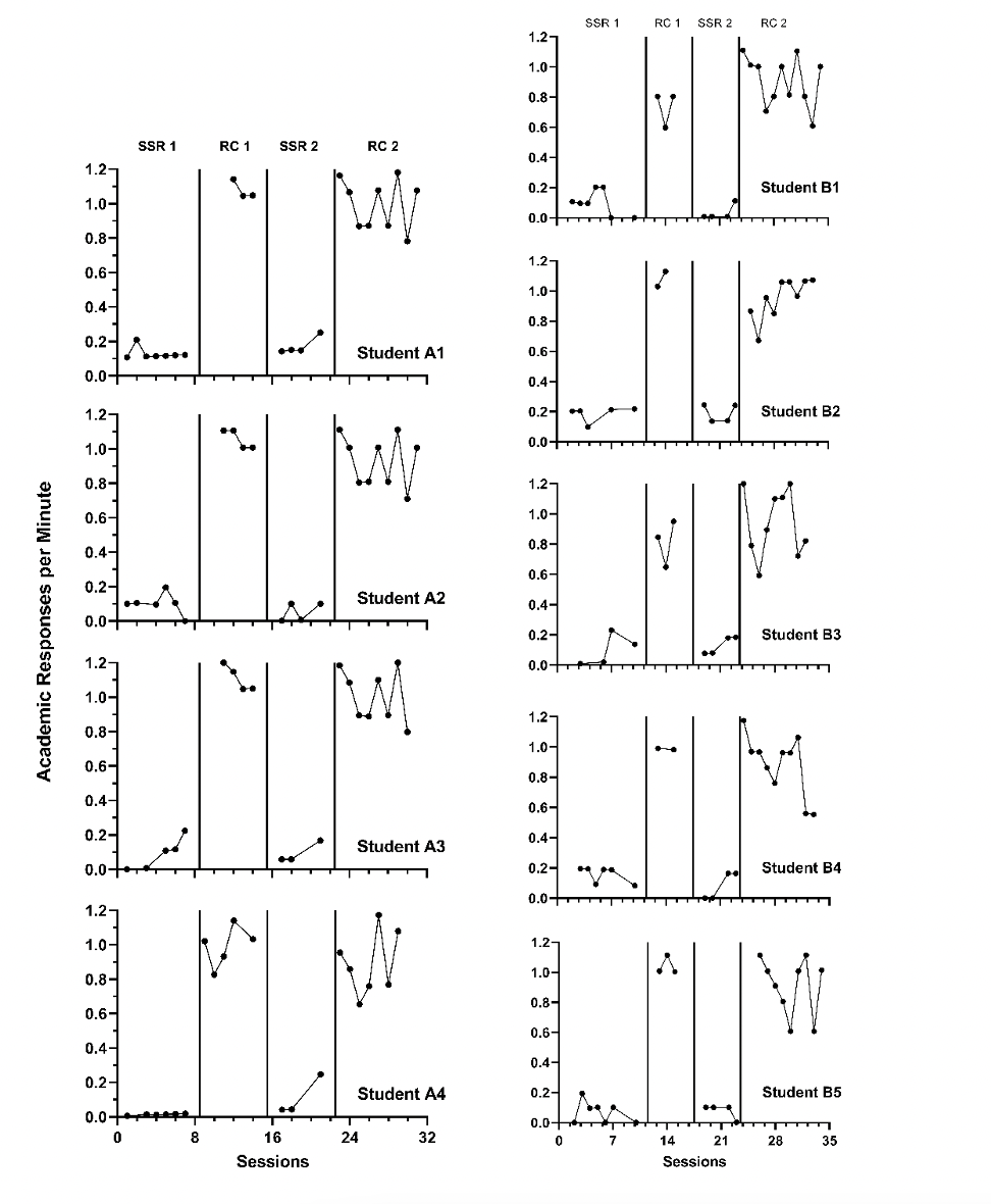
Figure 3.3: Replicated ABAB Data Extracted from Lambert et al. (2006)
3.2 Details of the No Trend Models for Design-Comparable Effect Sizes
To fully differentiate between Model 1 and Model 2, we present the formal specification of each. For both Model 1 and Model 2, we can write the within-case model as: \[\begin{equation} \tag{3.1} Y_{ij} = \beta_{0j} + \beta_{1j}Tx_{ij} + e_{ij}, \end{equation}\] where \(Y_ij\) is the score on the outcome variable \(Y\) at measurement occasion \(i\) for case \(j\), and \(Tx_{ij}\) is dummy coded with a value of 0 for baseline observations and a value of 1 for the treatment phase observations. The mean baseline level for case \(j\) is \(\beta_{0j}\) (see Figure 3.4 for a visual representation of \(\beta_{0j}\) and \(\beta_{1j}\)). The raw score treatment effect for case \(j\) is indexed by \(\beta_{1j}\), which is the difference between the treatment phase outcome mean and the baseline phase mean. The error (\(e_{ij}\)) is time- and case-specific and assumed normally distributed and first-order autoregressive with variance \(\sigma_e^2\).
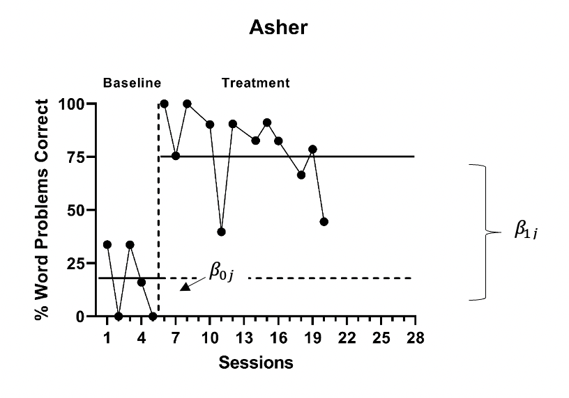
Figure 3.4: Illustration of Treatment Effect for Asher (Peltier et al., 2020)
For Model 1, the between-case model is: \[\begin{equation} \tag{3.2} \beta_{0j} = \gamma_{00} + u_{0j} \end{equation}\] \[\begin{equation} \tag{3.3} \beta_{1j} = \gamma_{10} \end{equation}\] where \(\gamma_{00}\) is the across-case average baseline mean and \(u_{0j}\) is a case-specific error, which is the deviation from the overall average for case \(j\). We assume the error is normally distributed with variance \(\sigma_{u_0}^2\). We assume the across-case average raw score treatment effect, \(\gamma_{10}\), to be constant for all cases. Thus, there is no error term in the equation for \(\beta_{1j}\). Based on this model, the design-comparable effect size is defined as the average raw score treatment effect (\(\gamma_{10}\)) divided by a SD that is comparable to the SD used to standardize mean differences in group-design studies (Pustejovsky et al., 2014): \[\begin{equation} \tag{3.4} \delta = \frac{\gamma_{10}}{\sqrt{\sigma_{u_0}^2 + \sigma_e^2}} \end{equation}\]
The Model 2 specification is like Model 1, with the only difference being an error term (\(u_{1j}\)) added to Equation (3.3) to account for between-case variation in the treatment effect. More specifically: \[\begin{equation} \tag{3.5} Y_{ij} = \beta_{0j} + \beta_{1j}Tx_{ij} + e_{ij}, \end{equation}\] \[\begin{equation} \tag{3.6} \beta_{0j} = \gamma_{00} + u_{0j} \end{equation}\] \[\begin{equation} \tag{3.7} \beta_{1j} = \gamma_{10} + u_{1j} \end{equation}\] Again, the across-case average baseline mean is \(\gamma_{00}\) and the across-case average raw score treatment effect (i.e., difference in treatment and baseline phase means) is \(\gamma_{10}\). The case-specific errors (\(u_{0j}\) and \(u_{1j}\)) account for between-case differences in baseline level and response to treatment. They are assumed multivariate normal with covariance \(\Sigma_u = \begin{bmatrix} \sigma_{u_0}^2 & \\ \sigma_{u_1u_0} & \sigma_{u_1}^2 \\ \end{bmatrix}\). We define the design-comparable effect size exactly as in Equation (3.4), because the effect size is scaled by the SD of the outcome in the absence of intervention and not dependent on the addition of \(u_{1j}\), which only impacts between-case variance in the treatment phase.
Because we tentatively selected Model 2 based on our a priori considerations, we use it to illustrate the estimation of design-comparable effect sizes for this data set. For several reasons, we also contrast the Model 2 results to what we obtain from Model 1. First, contrasting Model 1 and 2 results provides us with an additional way to examine the empirical support for our model selection. For instance, we could report that visual analyses of the model-implied individual trajectories for Model 2 fit the raw data better than the model implied individual trajectories from Model 1. Second, the contrast allows us to examine the sensitivity of our effect size estimates to the model chosen. For instance, this contrast may lead us to rule out between-case effect size variation as having a large impact on the estimated design-comparable effect size. Finally, contrasting allows us to illustrate a method of selecting between models in circumstances where a priori information is not sufficient.
3.3 Estimating the Design-Comparable Effect Size for the Single-Case Studies
3.3.1 Example 1: Multiple Baseline Study by Case et al. (1992)
We can estimate design-comparable effect sizes for all models suggested in Figure 3.4, using a web-based calculator for design-comparable effect sizes (scdhlm; Pustejovsky et al. (2021)). The scdhlm app is available at https://jepusto.shinyapps.io/scdhlm/. To use this app, researchers must store their dataset in an Excel file (.xlsx), comma delimited file (.csv), or text file (.txt). In addition, we recommend that users inspect their data to ensure the inclusion of the following variables: case identifier, phase identifier, session number, and the outcome. Although not required, researchers may want to arrange the data columns by order of variable appearance in the app. We show this arrangement for the Case et al. (1992) study in Figure 3.5. There, we demonstrate the following order of column headers with case identifier representing data in the first column, followed by variables in this order (left-to-right): phase identifier, session number, and the outcomes in the fourth column. Researchers have the flexibility to use any labeling scheme that clearly distinguishes between baseline and intervention conditions. For example, for the phase identifier, one can use \(b\) or 0 to indicate baseline observations and \(i\) or 1 to indicate intervention observations. However, the app requires that numerical values be used for both session number and outcome. Finally, we recommend that users arrange the data first by case (i.e., enter all the rows of data for the first case before any of the rows of data for the second case) and then by session number.
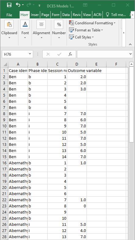
Figure 3.5: Illustration of Treatment Effect for Asher (Peltier et al., 2020)
After starting the app, we use the Load tab to load the data file, as illustrated in Figure 3.6. As mentioned previously, the data file can be a .txt or .csv file that includes one dataset, or an Excel (.xlsx) file that has either one (e.g., a data set for one study) or multiple spreadsheets (one spreadsheet for each of several studies). If using a .xlsx file with multiple spreadsheets, the scdhlm app allows us to select the spreadsheet containing the data for the study of interest from the Load tab. Then, we use the drop-down menus on the right of the screen to indicate the study design (treatment reversal versus Multiple Baseline/Multiple Probe across participants) and which variables in the data set correspond to the case identifier, phase identifier, session, and outcome (see Figure 3.6).
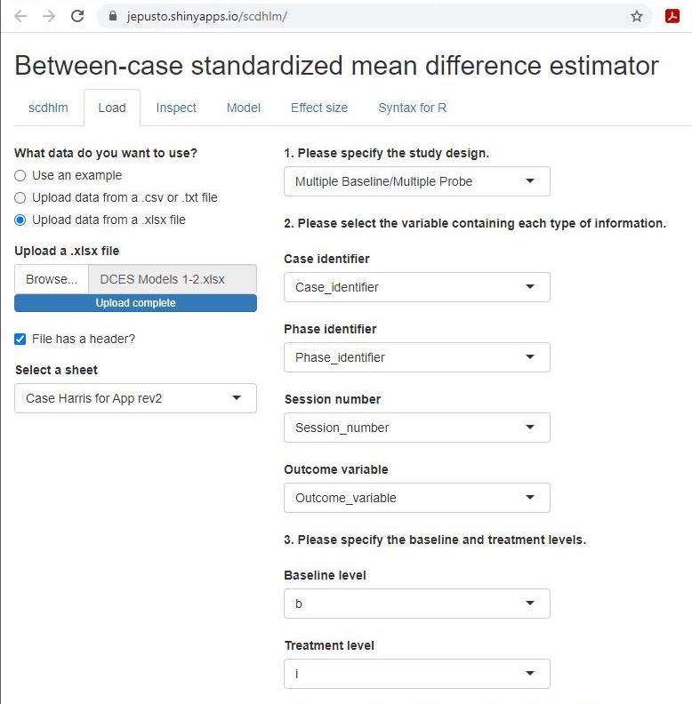
Figure 3.6: Between-Case Standardized Mean Difference Estimator (scdhlm, v. 0.6.0) Load Tab
After loading our data, we use the Inspect tab to ensure the accurate import of raw data into the app and assigned variable names are accurate (Figure 3.7). In addition, we can use the Inspect tab to view a graph of the data (Figure 3.8). We recommend that researchers compare these data with the graphed data from the original studies to ensure accuracy in uploading the data and specifying the design and variable names on the Load tab. Check the graphed data again for consistency with the (tentatively) selected model for the design-comparable effect size.
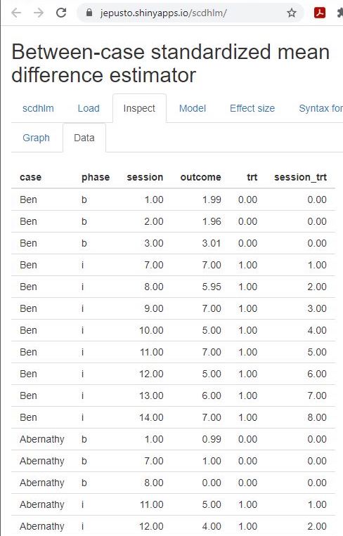
Figure 3.7: Between-Case Standardized Mean Difference Estimator (scdhlm, v. 0.6.0) Data Tab within Inspect Tab for Case et al. (1992)
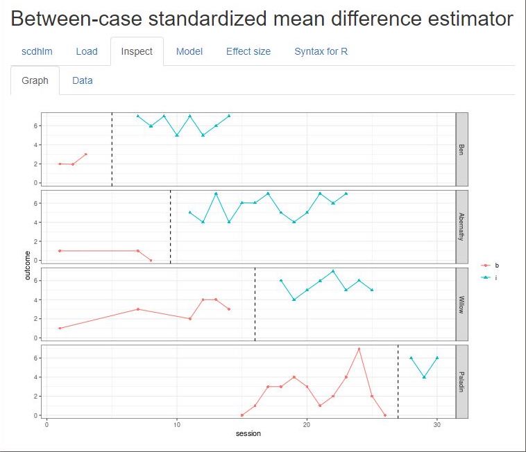
Figure 3.8: Between-Case Standardized Mean Difference Estimator (scdhlm, v. 0.6.0) Graph Tab Within Inspect Tab for Case et al. (1992)
After inspecting the data, we next specify the model for the design-comparable effect size using the Model tab. Figure 3.9 shows our specification for Model 2 (i.e., the model that assumes no trends and an effect that varies across cases). The specification process begins with the selection of trend type for the baseline phase. For this example, under Type of time trend, we select level because we assume no time trends in the baseline phases. Then, we opt to include level as a fixed effect and check the box to enable the model estimation of the average baseline level (i.e., \(\gamma_{00}\) from Equation (3.6)). We also include level as a random effect, so that the baseline level can vary from case to case. Focusing on the treatment phase next, we select change in level as the Type of time trend, because we assume that the treatment will only change the level of the outcome (not trend) and include change in level as a fixed effect. As a fixed effect, we can obtain an estimate of the average shift in level between baseline and treatment phases (i.e., \(\gamma_{10}\) from Equation (3.7). Finally, we choose to include change in level as a random effect to allow the change in level (i.e., treatment effect) to vary from case to case. Note the scdhlm app allows us to make different potential assumptions about the correlation structure of the session-level errors. Shown in Figure 3.9 are the default options of auto-regautoregressive and constant variance across phases. These defaults match the model presented in Equation (3.1). At this point, our model for the design-comparable effect size matches Model 2 from Figure 2.4.
At the bottom of the screen, the scdhlm app provides a graph of the data with trend lines based on the specified model. We recommend that users inspect this graph to ensure that the trend lines fit the data reasonably well. If the trend lines do not fit the data well, a question about model selection arises. For example, we find the baseline trend line for Abernathy is relatively high compared to their actual baseline observations. However, other model specifications (e.g., Model 1 shown later) did not improve the fit of Abernathy’s baseline trend line. So, we decide to proceed with estimation because most other trend lines look appropriate, and the model is consistent with our a priori expectations. Throughout this process, researchers should maintain a high standard for transparency in decision-making when reporting methods and results.
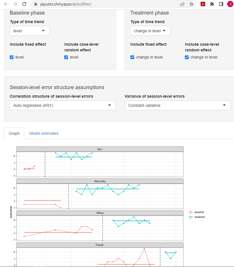
Figure 3.9: Between-Case Standardized Mean Difference Estimator (scdhlm, v. 0.6.0) Model Tab Showing Model 2 Specification for Case et al. (1992)
For the Case et al. (1992) data set, the a priori-identified Model 2 provides trajectories that fit the data reasonably well1. Thus, we proceed to the Effect size tab. As shown in Figure 3.10, the estimated design-comparable effect size for this study is 2.57 with a standard error (SE) of 0.45 and \(95\%\) confidence interval (CI) [1.65, 3.50].
Additional information reported on the Effect size tab include estimates of other quantities from the model, information about the model specification, and the assumed time-points used in calculating the design-comparable effect size. The reported degrees of freedom are used in making a small-sample correction to the effect size estimate, analogous to the Hedges’ g correction used with group designs (Hedges, 1981). Larger estimated degrees of freedom imply more precision in estimating the denominator of the design-comparable effect size, making the small-sample correction less consequential. Conversely, smaller degrees of freedom are indicative of imprecise design-comparable effect size denominator estimation, making the small-sample correction more consequential. The Effect size tab, shown in 3.10, also reports autocorrelation, which is the estimate of the correlation between level-1 errors of the model for the same case, differing by one time point (i.e., session) based on a first-order autoregressive model. Given the selected follow-up time, the reported intra-class correlation is an estimate of the between-case variance of the outcome as a proportion of the total variation in the outcome (including both between-case and within-case variance). Larger values of the intra-class correlation indicate that more of the variation in the outcome is between participants. The remaining output information (Study design, Estimation method, Baseline specification, Treatment specification, Initial treatment time, Follow-up time) describe the model specification and assumptions used in the effect size calculations. The scdhlm app includes such to allow for reproducibility of the calculations.
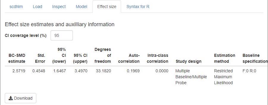
Figure 3.10: Between-Case Standardized Mean Difference Estimator (scdhlm, v. 0.6.0) Effect size Tab Showing Model 2 Estimate for Case et al. (1992)
If our a priori arguments for selecting Model 2 were weak, or we wanted to consider Model 1, we can easily compute the results of a different model by going back to the Model tab and changing our specification. The only difference is that Model 1 does not include change in level as a random effect for the treatment phase. For illustration purposes, we present Model 1 specification results for this study in Figure 3.11. As before, we keep the level option selected as the Type of time trend for the baseline phase, as both a fixed effect and a random effect. In the treatment phase, we keep change in level as the Type of time trend but select only change in level as a fixed effect. The Model 1 trend lines fit similarly to those from Model 2; the Model 1 design-comparable effect size is 2.59 with an SE of 0.41 and \(95\%\) CI [1.76, 3.42]. This suggests that the effect size estimate is not sensitive to our decision about whether the treatment effect varies across cases. Despite this information, we proceed with the Model 2 estimate because it is consistent with our expectations for the research in this area.
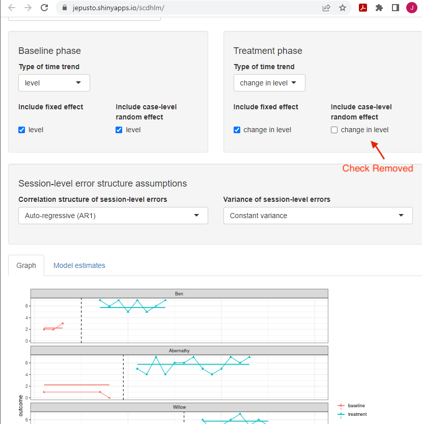
Figure 3.11: Between-Case Standardized Mean Difference Estimator (scdhlm, v. 0.6.0) Model Tab Showing Model 1 Specification for Case et al. (1992)
3.3.2 Example 2: Multiple Baseline Study by Peltier et al. (2020)
We now have a design-comparable effect size for the first single-case study by Case et al. (1992). Next, we repeat these steps for all other SCD studies in our synthesis. For this illustration, we include a second multiple baseline study (Peltier et al., 2020). For this second study, we ran through the same sequence of steps: 1. load the data; 2. inspect the data in both tabular and graphic form; 3. specify our selected model for the data (i.e., Model 2 for this illustration); and 4. estimate the design-comparable effect size.
After performing these steps, we found that the estimated model trajectories for the Model 2 specification fit the Peltier et al. (2020) data well, as shown in Figure 3.12. For the Peltier et al. (2020) study, the design-comparable effect size is 2.95 with an SE of 0.28 and \(95\%\) CI [2.42, 3.53]. We then estimated the effect for Model 1 (i.e., we remove the check next to change in level under include random effect), which is the more restrictive model that does not allow the treatment effect to vary across cases. Model 1 produced a design-comparable effect size estimate of 2.83 with an SE of 0.24 and \(95\%\) CI [2.34, 3.31], like the Model 2 design-comparable effect size.
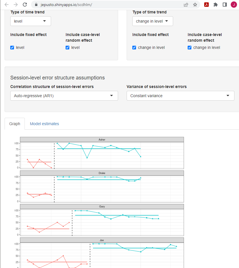
Figure 3.12: Between-Case Standardized Mean Difference Estimator (scdhlm, v. 0.6.0) Model 2 Specification for Peltier et al. (2020)
3.3.3 Example 3: Replicated ABAB Design by Lambert et al. (2006)
For the third SCD study, we illustrate use of the scdhlm app using data from a replicated ABAB design by Lambert et al. (2006). As with the previous two SCD studies, we load our spreadsheet containing the study data in the usual manner. However, unlike Case et al. (1992) and Peltier et al. (2020), the Lambert et al. (2006) study does not utilize a multiple baseline design. Therefore, on the right side of the Load tab, using the drop-down menu under Please specify the study design, we must select Treatment Reversal (as opposed to Multiple baseline/Multiple probe across participants). After loading the data, we again use the Inspect tab to visually inspect the data in both tabular and graphic form. Then using the Model tab (shown in Figure 3.13), we continue to specify Model 2 by checking the option under the Baseline phase to include level as both a fixed effect and a random effect and checking under the Treatment phase to include change in level as both a fixed effect and a random effect. Users of the app will note that for reversal designs, there is no drop-down menu from which they can potentially add trends (i.e., level is the only option for baseline specification, and change in level is the only option for treatment phase specification). This makes specification using the Model tab simpler than in our previous examples of multiple baseline studies, although it does also constrain the user’s ability to specify a well-fitting model. On the Model tab, we see that the fitted trajectories fit these data well.
After specifying the model, we view the Effect size tab to obtain the design-comparable effect size (see Figure 3.13). For Lambert et al. (2006), the estimated Model 2 design-comparable effect size is 6.37 with an SE of 0.39 and \(95\%\) CI [5.60, 7.14]. Like the previous SCD studies, we also estimate the effect for Model 1, which is the more restrictive model that does not allow the treatment effect to vary across cases. Model 1 produces an estimate of 6.34 with an SE of 0.37 and \(95\%\) CI [5.61, 7.08], a similar result to the Model 2 design-comparable effect size.
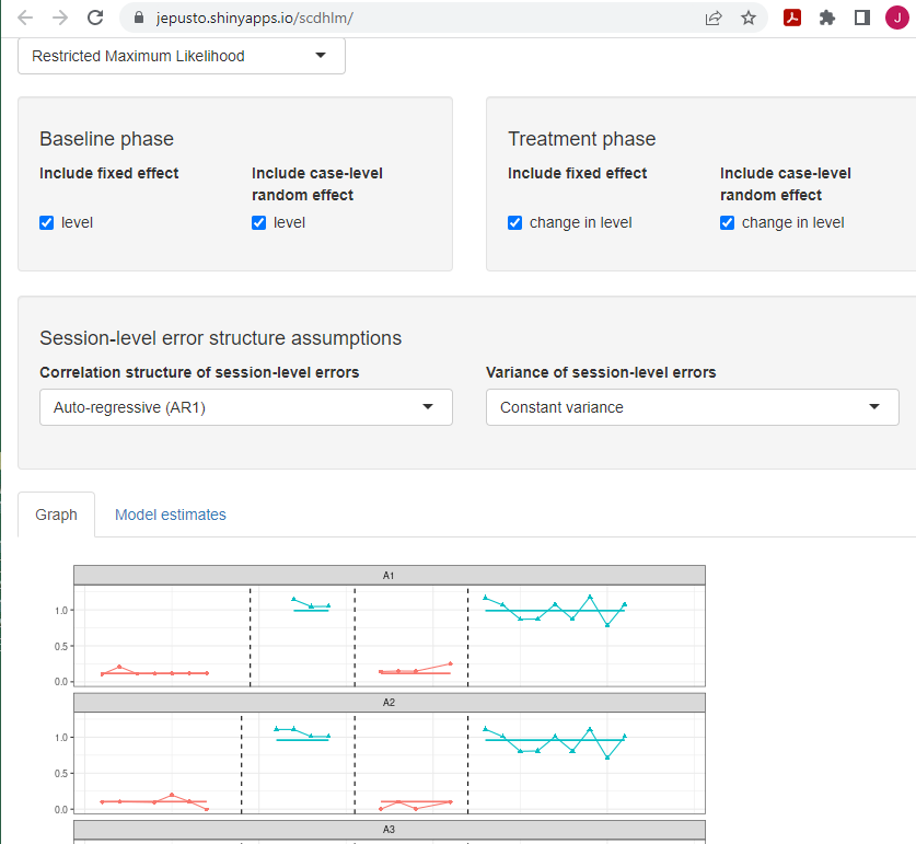
Figure 3.13: Between-Case Standardized Mean Difference Estimator (scdhlm, v. 0.6.0) Model 2 Specification for Lambert et al. (2006)
3.4 Estimating the Design-Comparable Effect Size for the Group Studies
After estimating the design-comparable effect size for each SCD study, we turn our attention to estimating the design-comparable effect size for each group study. Hutchinson (1993) used random assignment of individual students with learning disabilities to either the intervention (\(n = 12\)) or control (\(n = 8\)) conditions. After intervention, both groups of students completed 25 math word problems selected from the British Columbia Mathematics Achievement Test. Because details for estimating standardized mean difference effect sizes from group studies are readily available from a variety of sources including chapters (Borenstein, 2019), books (e.g., Borenstein et al., 2021) and journal articles (Hedges, 1981; e.g., Hedges, 2007), we do not model the calculation procedures and simply report the results. Using the Hutchinson (1993) group design study summary statistics at posttest, we calculate a standardized mean difference in math word problem solving as 0.71, with an SE of 0.45 based on Hedges’ g to correct for small-sample bias.
3.5 Analyzing the Effect Sizes
After we have obtained effect sizes from each single-case and group study, we can proceed with synthesizing the effect sizes. Depending on our synthesis goals, we have a variety of tools and approaches available. We can: (a) create graphical displays (e.g., forest plots) to show the effect size for each study along with their confidence interval, (b) average the effect sizes and create a confidence interval for the overall average effect, (c) estimate the extent of variation in effects across studies, (d) examine the effect sizes for evidence of publication bias, and (e) explore potential moderators of the effect. Since the use of design-comparable effect sizes for the SCD studies produce estimates having the same metric as the commonly used standardized mean difference effect sizes from group studies, researchers can accomplish these goals (e.g., averaging the effect sizes or running a moderator analysis) using methods developed for group studies. Details on these methods are readily available elsewhere (e.g., Borenstein et al., 2021; H. Cooper et al., 2019). We illustrate the averaging of the effect sizes from our studies here using a fixed effect meta-analysis, so that this illustration is consistent with the approach used in What Works Clearinghouse intervention reports (What Works Clearinghouse, 2020b).
Table 3.1 reports the effect size estimates, SEs, and fixed effect meta-analysis calculations for our four included studies. In fixed effect meta-analysis, the overall average effect size estimate is a weighted average of the effect size estimates from the individual studies, with weights proportional to the inverse of the sampling variance (squared SE) of each effect size estimate. Further, the SE of the overall effect size is the square root of the inverse of the total weight. In Table 3.1, column C reports the inverse variance weight assigned to each study, with the percentage of the total weight listed in parentheses. For instance, the effect size estimate from Peltier et al. (2020) receives 43.7% of the total weight, while the effect size estimates from Case et al. (1992) and Hutchinson (1993) each receive 16.9% of the total weight. The total inverse variance weight is 29.21. The overall average effect size estimate is 3.28 with an SE of 0.18 and an approximate \(95\%\) CI [2.91, 3.64]. The Q-test for heterogeneity is highly significant, Q(3) = 99.3, p < .0001, indicating that the included effect size estimates are more variable than we would expect due to sampling error alone. In other words, it is unlikely that we would observe such a wide dispersion of effect size estimates if the studies were all estimating the same true effect size parameter.
| Study | Effect Size Estimate (A) | Standard Error (B) | Inverse-variance Weight (%) (C) |
|---|---|---|---|
| Case et al. (1992) | 2.57 | 0.45 | 4.94 (16.9) |
| Peltier et al. (2020) | 2.95 | 0.28 | 12.76 (43.7) |
| Lambert et al. (2006) | 6.37 | 0.39 | 6.57 (22.5) |
| Hutchinson (1993) | 0.71 | 0.45 | 4.94 (16.9) |
| Fixed effect meta-analysis | 3.28 | 0.19 | 29.21 (100) |
In fixed effect meta-analysis, the overall average effect size estimate is a summary of the effect size estimates across the included studies, where studies are treated as fixed. Therefore, the SE and CI in fixed effect meta-analysis account for the uncertainty in the process of effect size estimation that occurs in each of the individual studies. However, they do not account for uncertainty in the process of identifying studies for inclusion in the meta-analysis (Konstantopoulos & Hedges, 2019; Rice et al., 2018), nor do they provide a basis for generalization beyond the included studies. When conducting syntheses of larger bodies of literature—and especially of studies with heterogeneous populations, design features, or dependent effect sizes—researchers will often prefer to use random effects models (Hedges & Vevea, 1998) or their further extensions (Pustejovsky & Tipton, 2021; Van den Noortgate et al., 2013).
Of the studies we use as illustrative examples in this chapter, the dependent variable of the group study (Hutchinson, 1993) was the broadest. Conversely, the Case et al. (1992) and Peltier et al. (2020) MB studies used more narrowly defined dependent variables. Finally, we note the outcome from the replicated ABAB design (Lambert et al., 2006) included a behavioral component (i.e., it is not purely academic). In a synthesis of many studies, researchers might use moderator analysis (i.e., meta-regression analysis) to explore the extent to which variation in effect size is related to dependent variable characteristics or other study features. Methods for conducting such moderator analysis are described elsewhere (Borenstein et al., 2021, Chapters 19–21; Konstantopoulos & Hedges, 2019).
References
Meta-analysis must specify their criteria for “reasonably well”.↩︎