Chapter 4 Illustration of Design-Comparable Effect Sizes When Assuming Only Trends in The Treatment Phases
This chapter illustrates the computation of design-comparable effect sizes in contexts where one assumes trends in the treatment phase only, with no trends in the baseline phase. Using data from two multiple baseline studies and a group study, we provide step-by-step instructions for selecting design-comparable effect sizes for the single-case studies and estimating them using the scdhlm app. We also briefly discuss estimating the effect size for the group study and synthesizing the effect sizes across the single-case and group and design studies.
In this chapter, we demonstrate the computation of design-comparable effect sizes using models with trends in the treatment phase(s) online (i.e., no baseline trend), as represented by Models 3 and 4 in Figure 2.4. These models assume that: (a) baseline observations of the dependent variable for each case occur at a stable level and (b) intervention leads to a change in both level and trajectory or growth rate in the treatment phase.
Let us consider a hypothetical scenario where we are interested in synthesizing single-case design (SCD) and group design studies that report intervention effects for reducing the amount of time it takes individuals to fall asleep at night (i.e., sleep onset latency). For purposes of illustration, we consider a review comprised of just three studies, including two multiple baseline designs and one group design. The first SCD study (Delemere & Dounavi, 2018) investigated the effects of two parent-implemented interventions (positive routines versus fading routines) on reducing sleep onset latency for six child participants with autism. Our second included SCD study, Gunning & Espie (2003), evaluated the effects of a sleep intervention on reducing the sleep latency of seven adult participants with intellectual disabilities. Our third study, a group design by Montgomery (2004), compared the efficacy of two sleep intervention delivery methods (face-to-face or booklet) for 66 children with learning disabilities (aged 2–8 years) randomly assigned to either treatment or waitlist control groups.
We recommend that researchers use the decision rules in Figure 1.1 to select a method to estimate and synthesize effects, and to consider design-comparable effect sizes when the purpose is to aggregate effects across SCD and group design studies. For Models 3 and 4 and using the aforementioned set of studies for our hypothetical synthesis, we break down the process of model selection and estimation into four steps: 1. Selecting a design-comparable effect size for the SCD studies. 2. Estimating the design-comparable effect size for the SCD studies using the scdhlm app (Pustejovsky et al., 2021). 3. Estimating the effect sizes for the group studies. 4. Synthesizing the effect sizes across single-case and group studies.
We focus on the first two steps because guidance and illustrations of methods for group studies are readily available from other sources (Borenstein et al., 2021; H. Cooper et al., 2019).
4.1 Selecting a Design-Comparable Effect Size for the Single-Case Studies
We begin by using the decision rules in Figure 2.4 to guide our selection of an appropriate design-comparable effect size. Across the studies, we use our knowledge of the population, context, and outcome of interest to inform any assumptions about the presence or absence of trends in either baseline and/or treatment phases. For our included studies, we assume that all participants generally have stable but high levels of behavior impeding a healthy nighttime routine (e.g., long latency to onset of sleep, frequent nighttime awakenings, etc.). We also assume no therapeutic trend in the baseline phase for each participant because otherwise there would be no need for the participants to receive the intervention. Further, we postulate that intervention will result in improved sleep behavior over time, as noted by a reduction in sleep problems in the treatment phase. Because we predict trend in only the treatment phase but not the baseline phase, we tentatively consider using Model 3 or Model 4 (see Figure 2.4).
Ideally, we would make the choice between Model 3 and Model 4 based on a logic model and a priori expectation of treatment effect variation (or lack thereof) within and across cases. For example, if we hypothesize that treatment effects do not vary from one case to the next, we will specify our design-comparable effect size using Model 3. Alternatively, if we assume that effects do vary across cases, we will use Model 4. For this synthesis, we note that all studies investigated sleep problems in the context of a participant’s own home. Furthermore, primary caregivers delivered the interventions, and we assume they have different learning histories and backgrounds. Therefore, we believe it is reasonable to anticipate some variation in the effect across cases and tentatively select Model 4.
The next step in the selection of design-comparable effect sizes for SCDs requires us to conduct visual inspection of each SCD study graph to see if our trend assumptions hold. We extracted data from the Delemere & Dounavi (2018) study and present the multiple baseline across participant graphs in Figure 4.1 (three participants who received the bedtime fading intervention) and Figure 4.2 (three participants who received the positive routines intervention). In Figure 4.3, we extracted data from the Gunning & Espie (2003) study and present the multiple baseline design graph for the seven participants with the target outcome of reducing sleep onset. When visually analyzing the graphs, we consider whether the data are reasonably consistent with the homogeneity and normality assumptions underlying any of the models for design-comparable effect sizes. In Figures 4.1-4.3, we observe similar variation between cases and variation across phases within each case and conclude that the assumption of homogeneous level-1 variance is tenable. In addition, we find no severe outlying data to suggest clear departures from non-normality. Therefore, our initial decision to use design-comparable effect sizes appears appropriate.

Figure 4.1: Multiple Baseline Data for Martin, Alan, and John (Delemere & Dounavi, 2018)

Figure 4.2: Multiple Baseline Data for Niahm, Mary, and Thomas (Delemere & Dounavi, 2018)
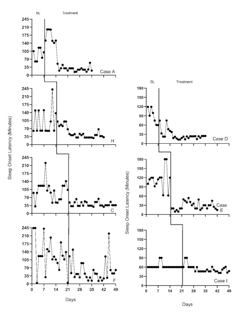
Figure 4.3: Multiple Baseline Design Data from 7 Participants with the Target Outcome of Reducing Sleep Onset Latency (Gunning & Espie, 2003)
Next, for our included studies, we consider the appropriateness of Models 3 and 4 that assume no trends in baseline. Visual inspection of the participants’ graphs in Figure 4.1 (Delemere & Dounavi, 2018) appears to reinforce our assumption of no trend in baseline data. Similarly, as shown in Figure 4.3 (Gunning & Espie, 2003), sleep onset latency neither increased nor decreased in the baseline condition for most participants. However, there are some exceptions to baseline stability observed. In Figure 4.3, Case D appears to show some improvement during baseline. In Figure 4.2, Niahm, Mary, and Thomas appear to have worsening sleep problems during the baseline phase. These trends are inconsistent with the typical pattern seen across cases in Figures 4.1 and 4.3. Whether there are truly trends that would continue is questionable. Perhaps the trends are artifacts related to fidelity or reliability of parental data collection, and thus would not continue.
In similar situations, we recommend that researchers reflect upon and reconsider their model selection. Using this specific example, it seems odd to assume that simply enrolling in a study would affect sleep patterns well established within the participant’s home routine. Rather, we find it more reasonable to assume that sleep onset latency for individuals with disabilities would vary around an average level across baseline observations. Therefore, we proceed with Model 4 because most cases in the included studies have baseline data consistent with the expectation of no trend, and because of the ambiguity and questions surrounding the few possible exceptions.
We proceed with visual inspection of observations in the treatment phase after examining baseline phase observations. Across most cases, we note an immediate change in the time it takes participants to fall asleep and a downward trend in treatment phase observations. While there are a few exceptions where participants appear to respond immediately to intervention, the downward trend does not continue across the remainder of the treatment phase (e.g., see Niahm, Mary, and Thomas in Figure 4.2). Because the design-comparable effect size assumes a common model across cases and estimates an average effect across the cases, we find it best to select a model that is consistent with the typical and expected pattern. Thus, it appears reasonable to proceed with a model that assumes no trend in baseline conditions and a trend in the treatment phase (i.e., Model 3 or Model 4 from Figure 2.4.
4.2 Details of the Models for Design-Comparable Effect Sizes
To appreciate how the treatment effect is defined in Models 3 and 4, let us examine the models in more detail. For both Model 3 and Model 4, we can write the within-case model as: \[\begin{equation} \tag{4.1} Y_{ij} = \beta_{0j} + \beta_{1j}Tx_{ij} + \beta_{2j}Tx_{ij}\times(Time_{ij}-k_j-D) + e_{ij}, \end{equation}\] where \(Y_{ij}\) is the score on the outcome variable \(Y\) at measurement occasion \(i\) for case \(j\), \(Tx_{ij}\) is dummy coded with a value of \(0\) for baseline observations and a value of \(1\) for the treatment phase observations, \(k_j\) is the last time-point before case \(j\) enters the treatment phase, and \(D\) is a centering constant that defines the focal time for indexing the treatment effect. The raw score treatment effect for case \(j\) is indexed by \(\beta_{1j}\), which is the distance between the treatment phase trend line and the baseline mean at the time where \((Time_{ij}-k_j-D)=0\). In Figure 4.4, we portray the raw score treatment effect for Martin at a time of 5 observations into treatment. If we set \(D<5\), the focal treatment effect would be smaller; if we set \(D>5\), the focal treatment effect would be larger. The other coefficients of the within-case model are \(\beta_{0j}\), which is the mean level of the outcome during baseline for case \(j\), and \(\beta_{2j}\), which is the slope of the treatment phase trend line for case \(j\). The error (\(e_{ij}\)) is time-specific and case-specific and assumed normally distributed and first-order autoregressive with variance \(\sigma_e^2\).
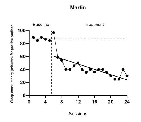
Figure 4.4: Martin’s Treatment Effect Five Observations into Treatment (Delemere & Dounavi, 2018)
Because the effect varies over time in the treatment phase and we estimate it at a specific focal time (i.e., when \((Time_{ij}-k_j-D)=0\)), it is important for us to consider what focal time we should select. For example, is it better to estimate the effect at the beginning of the treatment phase or between 3-10 observations into the treatment phase? Researchers should carefully consider their focal time selection by examining patterns in the typical treatment phase length in each SCD and group design study. For example, we chose to estimate the effect for the SCD studies 10 observations into the treatment phase for two reasons. First, 10 observations into treatment is closely aligned with the group design study time at posttest. Second, SCD studies in this area, like those used for this illustration, tend to have at least 10 treatment observations; a single exception in our studies can be seen for John (Delemere & Dounavi, 2018), who has only seven treatment observations.
For Model 3, the between-case model specification is: \[\begin{equation} \tag{4.2} \beta_{0j} = \gamma_{00} + u_{0j} \end{equation}\] \[\begin{equation} \tag{4.3} \beta_{1j} = \gamma_{10} \end{equation}\] \[\begin{equation} \tag{4.4} \beta_{2j} = \gamma_{20} \end{equation}\] where \(\gamma_{00}\) is the across- case average baseline mean and \(u_{0j}\) is a case-specific error, which accounts for variation between cases in their mean baseline levels and is assumes assumed to follow a normal distribution with variance \(\sigma_{u_0}^2\). We assume the same average treatment effect (\(\gamma_{10}\)) and the average slope for the treatment phase (\(\gamma_{20}\)) across cases. Thus, there are no error terms in the latter two equations. We show the design-comparable effect size in Equation (4.5), defined as the average raw score treatment effect (\(\gamma_{10}\)) divided by a standard deviation (SD) comparable to the SD used in group design studies. \[\begin{equation} \tag{4.5} \delta = \frac{\gamma_{10}}{\sqrt{\sigma_{u_0}^2 + \sigma_e^2}}, \end{equation}\]
Model 4 is specified in a very similar way as Model 3, apart from adding error terms (\(u_{1j}\) and \(u_{2j}\)) to the final two equations to account for between-case variation in the treatment effect and treatment phase slopes. More specifically: \[\begin{equation} \tag{4.6} Y_{ij} = \beta_{0j} + \beta_{1j}Tx_{ij} + \beta_{2j}Tx_{ij}\times(Time_{ij}-k_j-D) + e_{ij}, <!-- MC: I use Tx instead of Txt and use e_{ij} instead of r_{ij} in Equation 4.6 in the word doc.--> \end{equation}\] \[\begin{equation} \tag{4.7} \beta_{0j} = \gamma_{00} + u_{0j} \end{equation}\] \[\begin{equation} \tag{4.8} \beta_{1j} = \gamma_{10} + u_{1j} \end{equation}\] \[\begin{equation} \tag{4.9} \beta_{2j} = \gamma_{20} + u_{2j} \end{equation}\]
Again, the across-case average baseline mean is \(\gamma_{00}\) and the average raw score treatment effect at the focal time is \(\gamma_{10}\). The case-specific errors (\(u_{0j}, u_{1j}, u_{2j}\)), which account for between-case differences in baseline level and response to treatment, are assumed multivariate normal with covariance \(\Sigma_u = \begin{bmatrix} \sigma_{u_0}^2 & & \\ \sigma_{u_1u_0} & \sigma_{u_1}^2 & \\ \sigma_{u_2u_0} & \sigma_{u_2u_1} & \sigma_{u_2}^2\\ \end{bmatrix}\). Note that one could opt for a model that is intermediate between Model 3 and Model 4, by including only \(u_{1j}\) or \(u_{2j}\), and thereby allowing random variation in either (but not both) the level or slope changes. We proceed with random variability in each, because we think the treatment could lead to both different shifts in level and different treatment phase slopes for different participants. However, the inclusion of three random effects with an unstructured covariance matrix can be challenging to estimate with a limited number of cases. A simpler model with fewer random effects may be preferable if estimation difficulties arise.
Regardless of whether we allow both \(\beta_{1j}\) and \(\beta_{2j}\) to vary randomly as shown in Equations (4.8) and (4.9) or allow only one of these effects to vary randomly, we define the design-comparable effect size exactly as in Equation (4.5). This is because the effect size is scaled by the SD of the outcome in the absence of intervention (i.e., during baseline); it is not impacted by assumptions about the between-case variation during the treatment phase.
In the following sections, we will illustrate the estimation of design-comparable effect sizes for the SCD studies using Model 4 based on a priori considerations and the differences noted between cases in their treatment phase slopes. After obtaining the design-comparable effect sizes using Model 4, we repeat the process using Model 3 for several reasons. First, contrasting the models allows us an additional way to examine the empirical support for our chosen model. For instance, visual analyses of the model-implied individual trajectories for Model 4 might show a better fit than those for Model 3. Second, the contrast allows us to examine the sensitivity of the effect size estimates to our selected model. For instance, whether we assume the effect size varies across cases could have little to no effect on the design-comparable effect size estimate. Last, the contrast between Model 3 and Model 4 design-comparable effect sizes allows us to illustrate a method of selecting between models in circumstances where a priori information is not sufficient to select a model.
4.3 Estimating the Design-Comparable Effect Size for the Single-Case Studies
4.3.1 Example 1: Multiple Baselise Study by Gunning & Espie (2003)
We can estimate design-comparable effect sizes for any model in Figure 2.4 using a web-based calculator for design-comparable effect sizes (Pustejovsky et al., 2021). The scdhlm app is available at https://jepusto.shinyapps.io/scdhlm/. To use this app, researchers must store the data in an Excel file (.xlsx), comma delimited file (.csv), or text file (.txt). In addition, the data must include columns for the case identifier, +phase identifier_, session number, and outcome. Although not required, we suggest that researchers arrange their data columns by order of variable appearance in the scdhlm app, putting the case identifier in the first column, phase identifier in the second column and so on. We present this layout in Figure 4.5, representing data extracted for the study by Gunning & Espie (2003). In this illustration, for phase identifier, we use b to indicate baseline observations and i to indicate intervention observations. However, researchers can use any other labeling scheme that clearly distinguishes between baseline and intervention conditions (e.g., 0 and 1, respectively). Unlike the phase identifier variable, session number and outcome variables must contain numerical values. We also recommend entering data into the spreadsheet first by case (e.g., enter all the rows of data for the first case before any of the rows of data for the second case), then by session number.
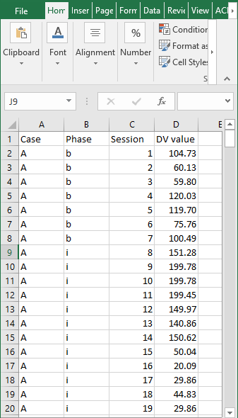
Figure 4.5: Snapshot of Spreadsheet Containing Extracted Gunning & Espie (2003) Data
After starting the app, we use the Load tab to load the data file, as illustrated in Figure 4.6. The data file could be a .txt or .csv file that includes one dataset or could be an Excel (.xlsx) file that has either one spreadsheet (e.g., a data set for one study), or multiple spreadsheets (one spreadsheet for each of several studies). If using a .xlsx file with multiple spreadsheets, we can select the spreadsheet containing the data for the study of interest from the Load tab. Then, we use the drop-down menus on the right of the screen to indicate the study design (Treatment Reversal versus Multiple Baseline/Multiple Probe across participants) and define which variables in the data set correspond to the case identifier, phase identifier, session, and outcome (see Figure 4.6).
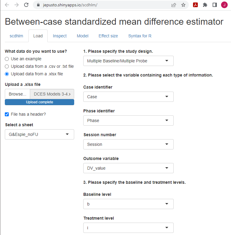
Figure 4.6: Between-Case Standardized Mean Difference Estimator (scdhlm, v. 0.6.0) Load Tab for Gunning & Espie (2003)
After we load our data, we use the Inspect tab to ensure that the raw data imported correctly and mapped to their corresponding variable names (Figure 4.7). In addition, we can use the Inspect tab to view a graph of the data (Figure 4.8). At this point, we recommend that researchers compare these data with the graphed data from the original studies as an additional measure that ensures the study data uploaded to the app correctly (according to the selections on the Load tab). Later, these graphed data can also be checked again for consistency with the tentatively selected model for estimating the design-comparable effect size.
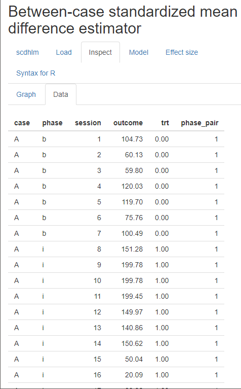
Figure 4.7: Between-Case Standardized Mean Difference Estimator (scdhlm, v. 0.6.0) Data Tab within the Inspect Tab for Gunning & Espie (2003)
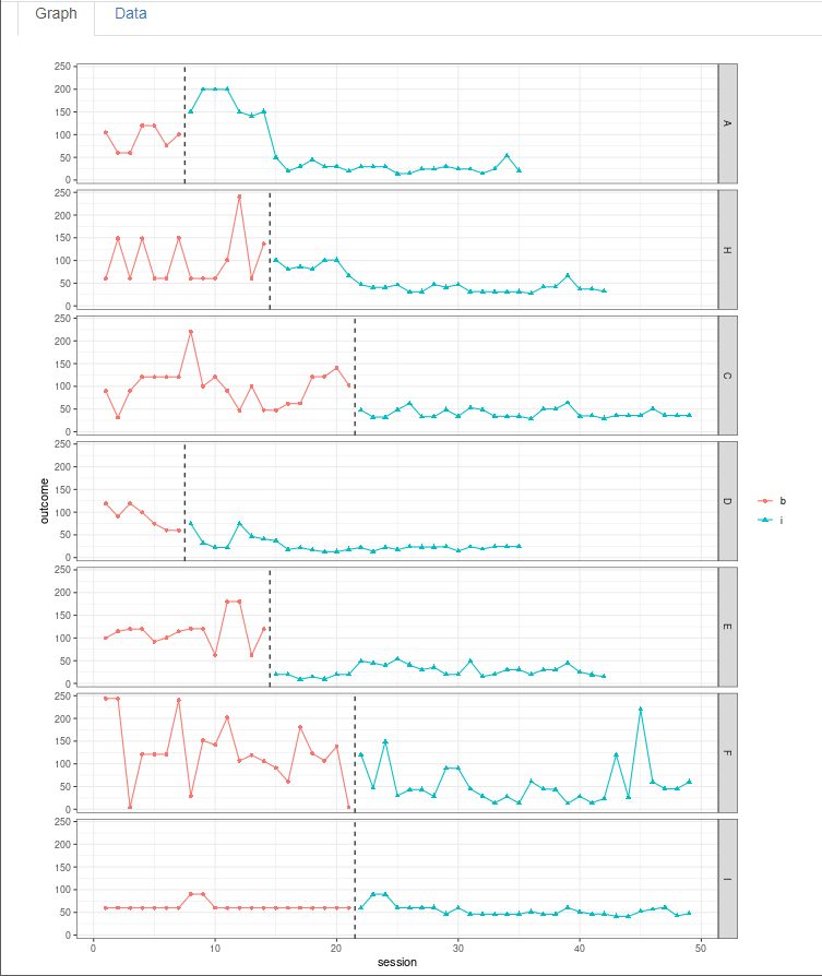
Figure 4.8: Between-Case Standardized Mean Difference Estimator (scdhlm, v. 0.6.0) Graph Display within the Inspect Tab for Gunning & Espie (2003)
Upon completion of data inspection, we next specify the model for the design-comparable effect size using the Model tab. Figure 4.9 shows the specification for Model 4, the model that assumes no baseline trend, a trend in the treatment phase, and an effect that varies across cases. Specification begins with the Baseline phase section, where we select level under Type of time trend because we assume that there are no time trends in the baseline phases. We then choose to include level as a fixed effect, enabling the model to estimate the average baseline level. We also include level as a random effect so that the baseline level can vary from case to case.
Next, we specify the model for the Treatment phase. In Type of time trend, we choose the option change in linear trend because Models 3 and 4 allow for possible time trends in only the treatment phases, implying that the trend changes across phases. To specify Model 4, we include both change in level and change in linear trend as fixed effects, so that the average trajectory across cases can reflect both an immediate change in level plus a change in the trend. We also select the option to include change in level as a random effect to allow the shift in level (i.e., treatment effect) to vary across cases. In addition, we opt to allow the change in linear trend to vary from case to case by including it as a random effect. At this point, we have specified the model for the design-comparable effect size that matches Model 4. Note the app allows us to make different potential assumptions about the correlation structure of the session-level errors. Shown are the default options of autoregressive and constant variance across phases. These defaults match the model presented in Equations (4.1) and (4.6) and are used because they seem appropriate for this data set. Also note that at the bottom of the screen (see Figure 4.9), the scdhlm app provides a graph of the data with trend lines that are based on the specified model (Figure 4.9). We recommend that researchers inspect this graph to ensure that the trend lines fit the data reasonably well. If they do not, it raises questions about the model choice.
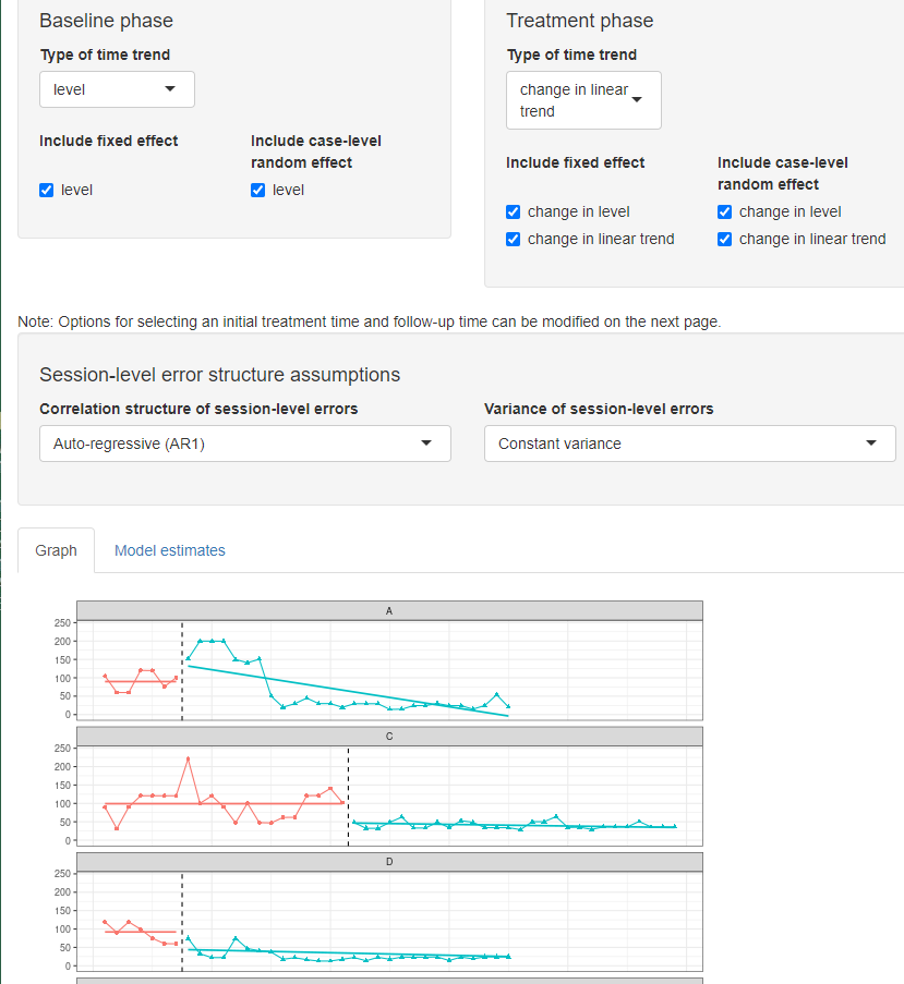
Figure 4.9: Between-Case Standardized Mean Difference Estimator (scdhlm, v. 0.6.0) Model 4 Specification for Gunning & Espie (2003)
For this data set, the a priori identified model provides trajectories that fit the data reasonably well, and thus we proceed to the Effect size tab (Figure 4.10). There are two sliders in the Hypothetical experimental parameters section above the effect size estimates output: Initial treatment time and Follow-up time. The numbers on each slider refer to the sessions or time points in the data series. Although the app populates times automatically, researchers can manipulate them manually to obtain an effect size estimate at a desired point in time. For models with trends in the baseline phase, it matters where we set the initial time. However, for models without baseline trends, only the distance between the two slider values matters.
We imagine a relatively typical SCD study with a baseline of 5; therefore, we use the sliding scale to set the Initial treatment time for the Gunning & Espie (2003) study to 5 to represent the last session before initiation of the treatment. Next, we estimate the treatment effect 10 observations into treatment and move the Follow-up time slider to the 15th observation. Given these Model 4 specifications for Gunning & Espie (2003), we find that the estimated between-case standardized mean difference 10 observations into treatment is -1.12 with a standard error (SE) of 0.34 and \(95\%\) confidence interval (CI) [-1.80, -0.45].
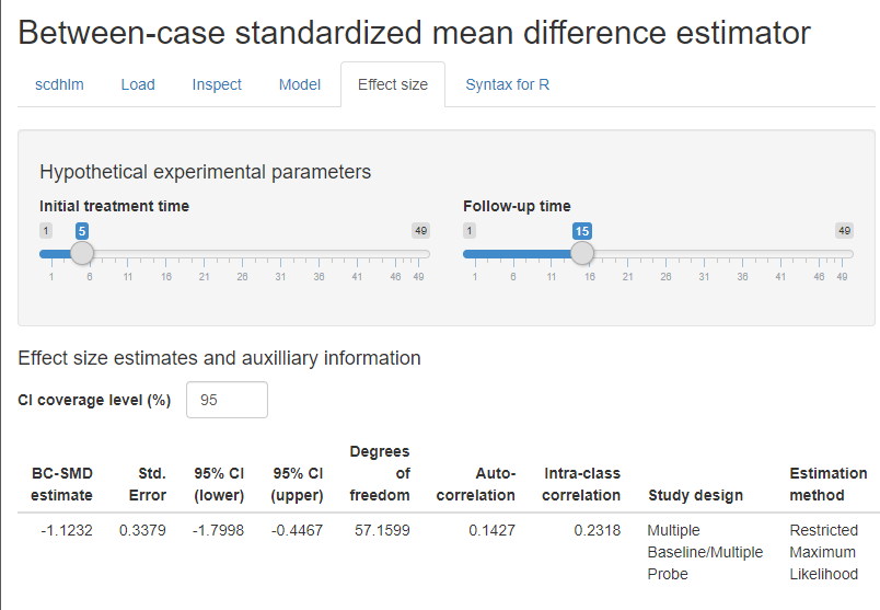
Figure 4.10: Between-Case Standardized Mean Difference Estimator (scdhlm, v. 0.6.0) Effect size Tab Showing Model 4 Estimate for Gunning & Espie (2003)
Now, if we lacked confidence in the a priori decision to select Model 4 and wanted to explore the Model 3 fit, we can re-run the study data without returning to the Load tab. Instead, we go directly to the Model tab to change our specification. To obtain Model 3, we remove (uncheck) change in level and change in linear trend as random effects, constraining the change in level and change in trend from baseline to treatment to be the same for each case. For Model 3, the estimated effect size is -1.10 with an SE of 0.17 and \(95\%\) CI [-1.43, -0.76]. In this case, for the Gunning & Espie (2003) study, the effect size estimates for both Models are similar. However, with the more restrictive assumptions of Model 3, the CI is narrower. If we had used a model that allowed a change in level to vary randomly, but required a fixed slope change, the estimated effect size would be -1.07 with an SE of 0.28 and 95% CI [-1.63, -0.51].
The Effect size tab (Figure 4.10) reports additional information including estimates of other model quantities, information about the model specification, and assumptions used in calculating the design-comparable effect size. The reported degrees of freedom are used by the app in making a small-sample correction to the effect size estimate, analogous to the Hedges’ g correction used with group designs (Hedges, 1981). Larger estimated degrees of freedom mean that the denominator of the design-comparable effect size is more precisely estimated, and that the small-sample correction is less consequential. Conversely, small degrees of freedom indicates that the denominator of the effect size is imprecisely estimated, making the small-sample correction more consequential. The reported autocorrelation is the estimate of the correlation between errors at the first level of the model for the same case that differ by one time-point (or session), based on a first-order autoregressive model. The reported intra-class correlation is an estimate of the between-case variance of the outcome as a proportion of the total variation in the outcome (including both between-case and within-case variance) as of the selected Follow-up time. Larger values of the intra-class correlation indicate that more of the variation in the outcome is between participants. The remaining information in the output (Study design, Estimation method, Baseline specification, Treatment specification, Initial treatment time, Follow-up time) describe the model specification and assumptions used in the effect size calculations. The app includes it to allow for reproducibility of the calculations.
4.3.2 Example 2: Multiple Baseline Study by Delemere & Dounavi (2018)
After obtaining a design-comparable effect size for the first SCD (Gunning & Espie, 2003), we repeat these steps for all other included SCD studies. In our second included SCD study (Delemere & Dounavi, 2018), the researchers analyzed two interventions. While we could estimate a separate design-comparable effect size for each, for the purposes of illustrating the computational steps in this chapter, we have pooled the data from the six cases to estimate one design-comparable effect size. To obtain a design-comparable effect size for the Delemere & Dounavi (2018) study, we follow the same sequence of steps: 1. Load the data. 2. Inspect the data in both tabular and graphic form. 3. Specify our selected model for the data (see Figure 4.11 for Model 4). 4. Estimate the design-comparable effect size.
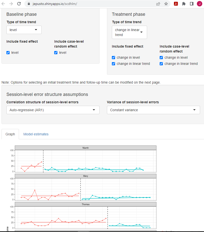
Figure 4.11: Between-Case Standardized Mean Difference Estimator (scdhlm, v. 0.6.0) Model 4 Specification for Delemere and Dounavi (2018)
Proceeding with Model 4, we use the Effect size tab of the scdhlm app to obtain a design-comparable effect size for the Delemere & Dounavi (2018) study. As with the previous example, the effect size will depend on the time into intervention at which we estimate the effect size the focal time (indicated by the scdhlm app variable named Follow-up time). When estimating design-comparable effect sizes for SCD studies, researchers should hold the Follow-up time constant across studies. Therefore, we use the Initial treatment time and Follow-up time sliders at the top of the screen to obtain an estimate of effect 10 observations into treatment (i.e., we set the Initial and Follow-up time sliders to five and 15, respectively). The resulting design-comparable effect size for the Delemere & Dounavi (2018) study is -0.70 with an SE of 0.33 and 95% CI [-1.49, 0.09].
Again, if we want to compare these results to those estimated using Model 3, we can go back to the Model tab to change our specification. To obtain Model 3, we remove (uncheck) change in level and change in linear trend as random effects to obtain the same change in level and change in trend from baseline to treatment across cases. We keep all other modeling options the same (e.g., Initial treatment time and Follow-up time). Figure 4.12 shows the Model 3 specification for the Delemere & Dounavi (2018) study. The estimated design-comparable effect size is -0.91 with an SE of 0.28 and 95% CI [-1.52, -0.29]. Comparing the fit of the trend lines obtained from Model 4 (Figure 4.11) to those from Model 3 (Figure 4.12), our originally specified Model 4 appears to provide a better fit for the primary study data. Because of this and because Model 4 is more consistent with both our a priori expectations and the data from our other SCD study (i.e., Gunning & Espie, 2003), it seems reasonable to proceed with the effect estimate from Model 4 (i.e., -0.70).
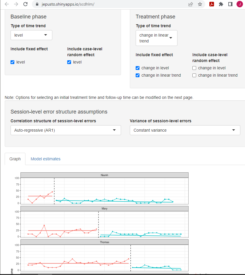
Figure 4.12: Between-Case Standardized Mean Difference Estimator (scdhlm, v. 0.6.0) Model 3 Specification for Delemere and Dounavi (2018)
4.4 Estimating the Design-Comparable Effect Size for the Group Studies
After estimating the design-comparable effect size for the included SCD studies, the next step is to estimate a design-comparable effect size for the included group design study. Details on estimating standardized mean difference effect sizes from group studies are readily available from a variety of sources, including Chapter 12 of The Handbook on Research Synthesis and Meta-Analysis (Borenstein, 2019), books (e.g., Borenstein et al., 2021) and journal articles (e.g., Hedges, 1981; Hedges, 2007). Therefore, we do not demonstrate the step-by-step effect size estimation methods for group design studies in this methods guide. Instead, we summarize the results below.
The included group design study, Montgomery (2004), reported a randomized trial comparing the efficacy of sleep interventions versus a wait-list control condition for families with children with severe learning disabilities. The researchers assigned participating families to a conventional face-to-face intervention (\(n = 20\)), a brief treatment delivered as a booklet (\(n = 22\)), or a wait-list control condition (\(n = 24\)). At posttest, the researchers compared participants’ composite sleep disturbance score (derived from parent reports) across groups, with higher scores corresponding to more severe sleep disturbance. For purposes of effect size calculations, we pooled the results from the face-to-face and booklet intervention conditions. Based on the post-treatment means and standard deviations (Montgomery, 2004, Table 1), the standardized mean difference in sleep onset at the end of intervention was -1.52, with an SE of 0.29. This effect size estimate is based on Hedges’ g, which corrects for small sample size bias.
4.5 Analyzing the Effect Sizes
As a final step, we synthesize the effect sizes across both SCD and group design studies. A variety of tools and approaches are available to researchers depending on the goals of their synthesis. For example, researchers can: (a) create graphical displays that show the effect size for each study along with its CI, (b) report an overall average effect size and CI by averaging effect sizes across studies and, (c) examine the extent of effect size variation across studies, (d) explore potential moderators of the effects, and (e) examine the effect sizes for evidence of publication bias. Because the use of design-comparable effect size for the SCD studies produces effect estimates that are like the commonly used standardized mean difference effect sizes from group studies, researchers can accomplish these goals using the methods already established for group design studies. Details on these methods are readily available elsewhere (e.g., Borenstein et al., 2021; H. Cooper et al., 2019). We illustrate the averaging of the effect sizes from our studies here using a fixed effect meta-analysis, consistent with the approach used in What Works Clearinghouse intervention reports (What Works Clearinghouse, 2020b).
Table 4.1 reports the effect size estimates, SEs, and fixed effect meta-analysis calculations for the example studies. The top panel uses the design-comparable effect size results for SCD studies based on Model 4. As a sensitivity analysis, the bottom panel presents the results based on Model 3. Note that the effect size estimate from the group design study is the same in both panels. In fixed effect meta-analysis, the overall average effect size estimate is a weighted average of the effect size estimates from the individual studies, with weights proportional to the inverse of the sampling variance (squared SE) of each effect size estimate. Further, the SE of the overall effect size is the square root of the inverse of the total weight.
Column C of Table 4.1 reports the inverse-variance weight assigned to each of the studies, with the percentage of the total weight listed in parentheses. In the top panel based on Model 4, the effect size estimate from the group design study receives \(40\%\) of the total weight, while the effect size estimates from the SCD studies receive \(29\%\) and \(31\%\) of the total weight, respectively. The total inverse variance weight is 29.72. The overall average effect size estimate based on Model 4 is -1.15 with an SE of 0.182 and an approximate 95% CI [-1.51, -0.79]. The Q-test for heterogeneity is not significant, \(Q(2) = 3.50\), \(p = .174\), indicating that the included effect size estimates are consistent with the possibility that all studies were estimating a common effect size parameter. Interestingly, in this example, the effect size estimate from the group design is larger in magnitude than the effect size estimates from the SCD studies.
| Study | Effect Size Estimate (A) | Standard Error (B) | Inverse-variance Weight (%) (C) |
|---|---|---|---|
| Model 4 | |||
| Gunning & Espie (2003) | -1.12 | 0.34 | 8.65 (29.1) |
| Delemere & Dounavi (2018) | -0.70 | 0.33 | 9.18 (30.9) |
| Montgomery et al. (2004) | -1.52 | 0.29 | 11.89 (40.0) |
| Fixed effect meta-analysis | -1.15 | 0.18 | 29.72 (100) |
| Model 3 | |||
| Gunning & Espie (2003) | -1.10 | 0.17 | 34.60 (58.4) |
| Delemere & Dounavi (2018) | -0.91 | 0.28 | 12.76 (21.5) |
| Montgomery et al. (2004) | -1.52 | 0.29 | 11.89 (20.1) |
| Fixed effect meta-analysis | -1.14 | 0.13 | 59.25 (100) |
The bottom panel of Table 4.1 reports the same calculations but using the design-comparable effect size estimates based on Model 3 for the two SCD studies. The most notable difference is that Model 3 more precisely estimates the design-comparable effect size for the Gunning & Espie (2003), resulting in more weight (\(58\%\)) assigned in the fixed effect meta-analysis. For Model 3, the overall average effect size is nearly identical to that obtained for Model 4 (-1.14), but the substantially smaller Model 3 design-comparable effect size for the Gunning & Espie (2003) study results in an SE of 0.13 and \(95\%\) CI [-1.40, -0.89].
In fixed effect meta-analysis, the overall average effect size estimate is a summary of the effect size estimates across the included studies, which are treated as fixed. Therefore, the SE and CI in fixed effect meta-analysis take into account the uncertainty in the process of estimating the effect sizes in each of the individual studies, but they do not account for uncertainty in the process of identifying studies for inclusion in the meta-analysis (Konstantopoulos & Hedges, 2019; Rice et al., 2018). Consequently, they do not provide a basis for generalization beyond the included studies. When conducting syntheses of larger bodies of literature—and especially of studies with heterogeneous populations, design features, or dependent effect sizes—researchers will often prefer to use random effects models (Hedges & Vevea, 1998) or their further extensions (Pustejovsky & Tipton, 2021; Van den Noortgate et al., 2013).
References
The SE of the overall effect size is the square root of the inverse of the total weight.↩︎