P-Value Selection Models for Meta-Analysis with Dependent Effects
James E. Pustejovsky
Megha Joshi
Martyna Citkowicz
2026-09-21
Source:vignettes/selection-models.Rmd
selection-models.RmdSystematic reviews and meta-analyses aim to provide comprehensive examinations of available evidence about phenomena of scientific or policy interest. One major challenge to this aim is selective reporting of evidence from primary studies. Selective reporting occurs when the direction or statistical significance level of a finding influences whether it is reported and therefore whether the finding is available for inclusion in a systematic review. If results that are positive and statistically significant are more likely to be reported than results that are null or negative, the evidence base available for meta-analysis will be distorted, leading to inflated effect size estimates from meta-analysis (Greenwald, 1975; Rothstein, Sutton, & Borenstein, 2005; Sutton, 2009) and biased estimates of heterogeneity (Augusteijn, van Aert, & van Assen, 2019).
Because selective reporting can make it difficult to draw accurate inferences from a meta-analysis, many tools have been developed that try to detect selective reporting problems and correct for the biases they create in meta-analytic summaries.1 Among these, selection models are a class of meta-analytic methods that provide both tests and bias-adjustments for selective reporting by directly modeling the section process (Citkowicz & Vevea, 2017; Hedges, 1992; Hedges & Vevea, 1996; Vevea & Hedges, 1995). However, few of the available methods for investigating selective reporting can accommodate dependent effect sizes. This limitation poses a problem for meta-analyses in education, psychology and other social sciences, where dependent effects are a common feature of meta-analytic data.
Dependent effect sizes occur when primary studies report results for multiple measures of an outcome construct, collect repeated measures of an outcome across multiple time-points, or involve comparisons between multiple intervention conditions. Further, dependence can also arise when meta-analyses include multiple primary studies conducted by the same researchers or the same lab (Pustejovsky & Tipton, 2022). This dependency violates statistical assumptions of independent errors, leading to overly narrow confidence intervals, hypothesis tests with inflated type one error rates, and incorrect inferences. Meta-analysts now have access to an array of methods for summarizing and modeling dependent effect sizes.2 These methods can be combined with a few of the available techniques for investigating selective reporting, but this is currently limited to techniques based on regression adjustment (Chen & Pustejovsky, 2024; Fernández-Castilla et al., 2019; Rodgers & Pustejovsky, 2020) or sensitivity analyses based on simple forms of selection models, which provide bounds on average effects given an a priori level of selective reporting (Mathur & VanderWeele, 2020).
The metaselection package expands the range of techniques available for investigating selective reporting bias while accommodating meta-analytic datasets that include dependent effect sizes.3
The metaselection package implements selection models based on step-function (Pustejovsky, Citkowicz, & Joshi, 2025) and beta-density (Citkowicz, Pustejovsky, & Joshi, 2026) selection processes.
Because these models describe the marginal distribution of effect size estimates, they bypass the computational complexity of modeling full multivariate dependence structures directly while still effectively reducing bias in average effect size estimates.
To account for dependent effect sizes, these models adjust standard errors after model fitting using either cluster-robust variance estimation (CRVE, i.e., sandwich estimation) or clustered bootstrapping.
Key takeaways and practical recommendations from simulation studies evaluating these methods (Citkowicz et al., 2026; Pustejovsky et al., 2025) include:
- Inference Method: Two-stage clustered bootstrapping consistently outperforms large-sample CRVE, providing close-to-nominal confidence interval coverage for the average effect size.
- Sample Size Requirements: A sample size of \(J \geq 30\) studies is generally needed for estimators to achieve low bias and for bootstrap confidence intervals to provide reliable coverage, particularly under severe selection.
- Bias–Variance Trade-off: While step-function and beta-density models substantially reduce systematic bias under selective reporting, this protection comes with a modest loss in efficiency compared to unadjusted estimates. This trade-off is particularly advantageous under more severe levels of selective reporting.
- Focus of Inference: Meta-analysts should primarily focus interpretation on the bias-adjusted average effect size (\(\mu\)). Selection parameters should be interpreted cautiously due to potential mis-calibration in their individual confidence interval coverage.
- Complementary Role: These models serve as flexible, parametric alternatives to regression adjustment or funnel plots, and their empirical selection estimates can also directly inform sensitivity analyses.
Selection Models
Selection models are a tool for investigating selective reporting by making explicit assumptions about the process through which the effect size estimates are reported (Rothstein et al., 2005).
Such models have two components: a set of assumptions describing the evidence-generation process and a set of assumptions describing the selection process.
The metaselection package implements a flexible class of selection models, in which the evidence-generating process follows a random effects location-scale meta-regression model (Viechtbauer & López‐López, 2022) and where the selection process is a function of one-sided \(p\)-values, either in the form of a step function (Vevea & Hedges, 1995) or a beta-density function (Citkowicz & Vevea, 2017).
The step function model involves specifying psychologically salient but functionally arbitrary thresholds (or steps), such as \(p < 0.05\), which categorize the \(p\)-values into intervals that have different probabilities of selection (Vevea & Hedges, 1995).
The beta-density model uses a different selection function, based on a beta distribution, to capture distinctive, more smoothly varying patterns of selection (Citkowicz & Vevea, 2017).
Consider a meta-analytic dataset with a total of \(J\) samples, where study \(j\) includes \(k_j\) effect size estimates. Let \(Y_{ij}\) denote an effect size estimate produced by a sample, prior to selective reporting. The effect size estimate has standard error \(\sigma_{ij}\), which is treated as a fixed quantity. Let \(\mathbf{x}_{ij}\) be a \(1 \times x\) row vector of predictors that encode characteristics of the effect sizes or the samples and may be related to average effect size magnitude. Let \(\mathbf{u}_{ij}\) be a \(1 \times u\) row vector of predictors that may be related to effect size heterogeneity. Let \(\Phi()\) denote the standard normal cumulative distribution function and \(\phi()\) the standard normal density. Finally, let \(p_{ij}\) be the one-sided \(p\)-value corresponding to the effect size estimate, which is a function of the effect size estimate and its standard error. For p-values computed under the alternative hypothesis that the effect size is positive, \(p_{ij} = 1 - \Phi\left(Y_{ij} / \sigma_{ij}\right) = \Phi\left(-Y_{ij} / \sigma_{ij}\right)\); for p-values computed under the alternative that the effect size is negative, \(p_{ij} = \Phi\left(Y_{ij} / \sigma_{ij}\right)\).
The evidence-generating process
The model for the evidence-generating process is a random effects location-scale meta-regression model, in which \[Y_{ij} = \mathbf{x}_{ij} \boldsymbol\beta + v_{ij} + e_{ij},\] where \(\boldsymbol\beta\) is a \(1 \times x\) vector of regression coefficients that relate the predictors to average effect size magnitude, \(v_i\) is a normally distributed random effect with mean zero and variance \(\tau^2_{ij}\), and \(e_{ij}\) is a normally distributed sampling error with mean zero and known variance \(\sigma^{2}_{ij}\). The variance of the random effects is modeled as \[\log\left(\tau_{ij}^{2}\right) = \mathbf{u}_{ij} \boldsymbol\gamma,\] where \(\boldsymbol\gamma\) is a \(u \times 1\) vector of coefficients that relate the predictors to the degree of marginal variation in the random effects. If the model does not include predictors of heterogeneity, then \(\mathbf{u}_{ij} = 1\) and the model reduces to a conventional random effects meta-regression in which \(\gamma = \log(\tau^2)\).
Note that this random-effects location scale model treats each observed effect size as if it were independent, even though the data may include multiple, statistically dependent effect size estimates generated from the same sample. Thus, it is a model for the marginal distribution of effect size estimates, which does not attempt to capture the dependence structure among effect size estimates drawn from the same sample. As a result, the regression coefficients \(\boldsymbol\beta\) describe the overall average effects (given the predictors) and variance parameters \(\boldsymbol\gamma\) describe the marginal or total heterogeneity of the effect size distribution, rather than decomposing the heterogeneity into within-sample and between-sample components.
Selective reporting processes
The selective reporting process is defined by a selection function, which specifies the probability that an effect size estimate is reported given its \(p\)-value. Let \(O_{ij}\) be an indicator for whether effect size \(i\) in study \(j\) is observed. Then the selection model defines \(\text{Pr}(O_{ij} = 1 \ | \ p_{ij}) = \text{Pr}(O_{ij} = 1 \ | \ Y_{ij}, \sigma_{ij})\). The package includes two different forms of selection functions: step functions and beta-density functions.
Although it is possible in principle to specify selection functions in terms of \(p\)-values from two-tailed hypothesis tests, the models implemented in the package are based on selection functions for one-tailed \(p\)-values. In primary studies, researchers typically report \(p\)-values from two-tailed hypothesis tests. However, prejudice against non-significant results is generally directional, and two-tailed \(p\)-values do not consider the sign or valence of the effect. Thus, our formulation and discussion of these functions uses one-tailed \(p\)-values for a pre-specified, directional alternative hypothesis.4
Step functions
Hedges (1992) and Vevea & Hedges (1995) proposed to model the selective reporting process using a step-function, with thresholds chosen to correspond to “psychologically salient” \(p\)-values. In the general formulation, suppose that there are \(H\) steps, \(\alpha_1,...,\alpha_H\), and that \[\text{Pr}(O_{ij} = 1 | p_{ij}) = \begin{cases} 1 & \text{if} & p_{ij} < \alpha_1 \\ \lambda_1 & \text{if} & \alpha_1 \leq p_{ij} < \alpha_2 \\ \lambda_2 & \text{if} & \alpha_2 \leq p_{ij} < \alpha_3 \\ \vdots \\ \lambda_H & \text{if} & \alpha_H \leq p_{ij}. \end{cases}\] The selection parameters \(\lambda_1,...,\lambda_H\) control the probabilities of selection given a \(p\)-value, with parameter \(\lambda_h\) defined as the relative probability that an effect size estimate is observed, given that its \(p\)-value is in the range \([\alpha_h, \alpha_{h+1})\), compared to the probability that an effect size estimate is observed, given that its \(p\)-value is in the range \([0, \alpha_1)\). The model is estimated in terms of log-transformed relative probabilities so that the parameter space is unrestricted, with \(\zeta_h = \log(\lambda_h)\), where \(-\infty < \zeta_h < +\infty\), for \(h=1,...,H\). With this parameterization, \(\zeta_1 = \cdots = \zeta_H = 0\) describes a process where effect sizes are reported with uniform probability regardless of their signs or statistical significance levels.
In practice, meta-analysts will often use only a small number of steps in the selection model. One common choice is the three-parameter selection model, which has a single step at \(\alpha_1 = 0.025\) (the default in the package), as depicted in 1. With this choice of threshold, positive effects that are statistically significant at the two-sided level of \(p < 0.05\) have a different probability of selection than effects that are not statistically significant or not in the anticipated direction.
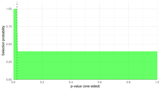
Figure 1: One-step selection model with \(\lambda_1 = 0.4\)
Another possibility is to use two steps at \(\alpha_1 = 0.025\) and \(\alpha_2 = 0.500\), which allows for different probabilities of selection for effects that are positive but not statistically significant and effects that are negative (i.e., in the opposite the intended direction). We call the latter model a four-parameter selection model; it is depicted in Figure 2.
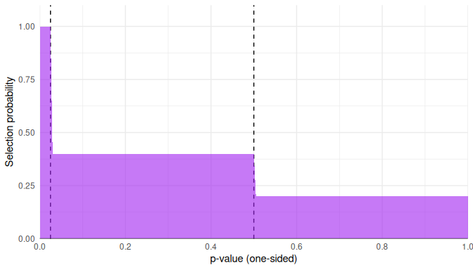
Figure 2: Two-step selection model with \(\lambda_1 = 0.4, \lambda_2 = 0.2\)
Beta-density functions
Citkowicz & Vevea (2017) proposed a selection model based on an alternative form of selection function, where the probability of reporting follows a beta density.
Compared to a step function, the beta density selection function can capture a very different set of shapes, with selection probabilities that vary smoothly over the range of possible one-sided \(p\)-values.
The metaselection package implements a modification of the beta-density function proposed in Citkowicz & Vevea (2017).
The modification involves truncating the selection probabilities at user-specified steps \(\alpha_1\) and \(\alpha_2\), so that the selection function is given by \[\text{Pr}(O_{ij} = 1 | p_{ij}) = \tilde{p}_{ij}^{(\lambda_1 - 1)} \left(1 - \tilde{p}_{ij}\right)^{(\lambda_2 - 1)},\] where \(\tilde{p}_{ij} = \min\{\max\{\alpha_1, p_{ij}\}, \alpha_2\}\).
Using this modification, one might set truncation points at \(\alpha_1 = 0.025\) and \(\alpha_2 = 0.975\) (the default values in the package) so that all statistically significant positive effect size estimates have the same selection probability and, likewise, all statistically significant, negative effect size estimates have the same selection probability, with the selection probabilities of non-significant effect sizes varying according to a beta density.
Figure 3 depicts this truncated beta density using the default truncation points and with \(\lambda_1 = 0.1, \lambda_2 = 0.9\), which represents very strong selection.
Figure 4 depicts a truncated beta density with more moderate values of \(\lambda_1 = 0.7, \lambda_2 = 1\) and where the second truncation point is set at \(\alpha_2 = 0.5\), so that all negative effect size estimates have equal selection probability.
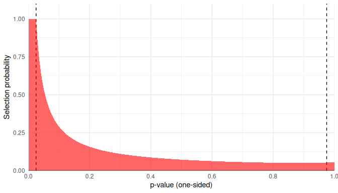
Figure 3: Beta-density selection model with \(\lambda_1 = 0.1, \lambda_2 = 0.9\), using truncation points \(\alpha_1 = 0.025, \alpha_2 = 0.975\)
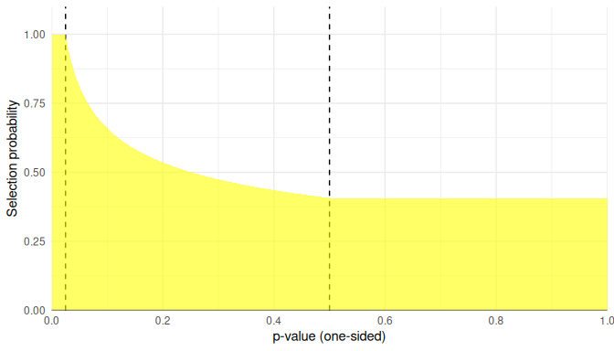
Figure 4: Beta-density selection model with \(\lambda_1 = 0.7, \lambda_2 = 1\), using truncation points \(\alpha_1 = 0.025, \alpha_2 = 0.500\)
In the package, the beta-density function is parameterized in terms of \(\zeta_h = \log(\lambda_h)\), where \(-\infty < \zeta_h < +\infty\), for \(h=1,2\). With this parameterization, \(\zeta_1 = \zeta_2 = 0\) describes a process where effect sizes are reported with uniform probability regardless of their statistical significance levels.
Estimation
The combination of assumptions about the evidence-generating process and assumptions about the selection process implies a marginal distribution for the observed effect sizes. The evidence-generating process describes the effect size distribution \(\text{Pr}(Y_{ij} = y_{ij} \ | \ \sigma_{ij}, \mathbf{x}_{ij}, \mathbf{u}_{ij})\) and the selection process specifies \(\text{Pr}(O_{ij} = 1 \ | \ Y_{ij} = y, \sigma_{ij}, \mathbf{x}_{ij}, \mathbf{u}_{ij})\). The distribution of observed effect size estimates then corresponds to \(\text{Pr}(Y_{ij} = y_{ij} \ | \ O_{ij} = 1, \sigma_{ij}, \mathbf{x}_{ij}, \mathbf{u}_{ij})\), which depends on the meta-regression coefficients \(\boldsymbol\beta\), the scale regression coefficients \(\boldsymbol\gamma\), and the selection parameters \(\boldsymbol\zeta\).
The metaselection package implements two different estimation strategies: penalized composite marginal likelihood (CML) and augmented and reweighted Gaussian likelihood (ARGL).
In smaller meta-analytic datasets or under conditions with severe selection where certain regions of the \(p\)-value distribution may have very sparse data, conventional maximum likelihood estimates of the selection parameter can be unstable or non-convergent.
To stabilize estimation under such conditions, both estimation functions allow specification of optional prior penalties on the parameters.
The specific penalties applied depend on the choice of selection function (step or beta) and the metric of the data (e.g., standardized mean differences, correlations, raw mean differences, log-odds ratios).
With CML estimation, model parameter estimates are obtained by finding the values that maximize the penalized log-composite-likelihood of the observations, treating each effect size estimate as if it were independent.
An alternative estimation strategy, augmented and reweighted Gaussian likelihood, defines the parameter estimator as the solution to a set of mean-zero estimating equations.
The selection parameters are estimated using their score equations, just as in the CML approach.
Unlike the CML strategy, the meta-regression coefficients and scale regression coefficients are estimated using the re-weighted log likelihood of the Gaussian evidence-generating process, with weights equal to the inverse probability of selection.
This strategy was initially suggested by Mathur & VanderWeele (2020), who focused on using inverse probability of selection weighting for purposes of sensitivity analysis with selection parameters specified a priori.
The implementation in the metaselection package uses the strategy to jointly estimate the meta-regression, scale regression, and selection parameters.
Pustejovsky et al. (2025)
Cluster-robust variance estimation
If each sample included in a meta-analysis provides just a single effect size estimate (i.e., if \(k_j = 1\) for \(j = 1,...,J\)), then standard errors and confidence intervals for the selection model parameters can be constructed using standard techniques based on the inverse of the Fisher information under the model.
Such an approach is used in other implementations of selection models, including the selmodel() function in the metafor package (Viechtbauer, 2010) and the weightfunct() function in the weightr package (Coburn & Vevea, 2019).5
However, this approach is predicated on the assumption that the effect size estimates are mutually independent.
Thus, it is inappropriate if the data include samples that provide multiple, statistically dependent effect size estimates.
For meta-regression models that do not account for selective reporting, Hedges et al. (2010) proposed CRVE methods (also known as sandwich estimators) that accommodate dependent effect sizes, even if the exact dependence structure is not known or is not correctly specified. The form of CRVE originally described in Hedges et al. (2010) is based on large-sample approximations and requires a relatively large number of independent samples (each of which might have multiple effect size estimates) to function well. Subsequent work developed small-sample refinements to CRVE, including adjustments to hypothesis tests and confidence intervals based on CRVE, which are accurately calibrated even for datasets that include a small number of independent clusters (Tipton, 2015; Tipton & Pustejovsky, 2015).
CRVE methods can also be applied to selection models to quantify uncertainty in parameter estimates obtained by penalized composite maximum likelihood or augmented and reweighted Gaussian likelihood.
The metaselection package provides standard errors and confidence intervals based on CRVE methods by default.
The implementation is similar to the original, large-sample CRVE methods described by Hedges et al. (2010); the subsequently developed small-sample refinements are not currently available for selection models.
It is important to bear in mind that CRVE methods are the default only because they are computationally convenient and quicker to compute compared to bootstrap-based methods—not because they are the best available method.
With CRVE, confidence intervals for model parameters can be constructed using large-sample normal approximations, but these intervals require a large number of independent samples to provide well-calibrated coverage levels.
Bootstrapped confidence intervals
A superior alternative to CRVE is to use bootstrap re-sampling methods to quantify uncertainty in parameter estimates.
Bootstrapping involves re-sampling many times from the original data to create an empirical distribution that can be used as a proxy for the actual sampling distribution of parameter estimates (Boos, 2003).
With dependent data structures, entire clusters of observations are re-sampled so that each bootstrapped dataset includes dependent observations, emulating the structure of the original dataset.
In the implementation in the metaselection package, this approach is called the multinomial bootstrap.
The package also implements two other variations of bootstrapping.
One variation, called the two-stage approach, re-samples clusters of observations and then re-samples effect size estimates within each cluster.
Another variation, known as the fractional random weight bootstrap (Xu, Gotwalt, Hong, King, & Meeker, 2020) or Bayesian bootstrap (Newton & Raftery, 1994; Rubin, 1981), involves assigning a random weight to each cluster of dependent observations, where the weights are simulated from an exponential distribution with mean 1.
Several different methods can be used to construct confidence intervals from a bootstrap distribution (Davison & Hinkley, 1997), which use various approximations and therefore vary in the accuracy of their coverage levels.
The metaselection package implements five different techniques, following the same methods and terminology as in the boot package (Canty & Ripley, 2021):
- The percentile confidence interval (
CI_method = "percentile") is based on quantiles of the bootstrap distribution. - The “basic” confidence interval (
CI_method = "basic") pivots the bootstrap distribution around the point estimate. - The bias-corrected and accelerated confidence interval (
CI_method = "BCa") adjusts the percentile confidence interval based on the bias of the sampling distribution and an “acceleration” adjustment for the relationship between the parameter and the variance of the estimator’s sampling distribution. - The standard normal confidence interval (
CI_method = "normal") uses the bootstrap standard error with a standard normal critical value. - The studentized confidence interval (
CI_method = "student") is based on the bootstrap distribution of the cluster-robust \(t\) statistic rather than the point estimator of a parameter.
Our simulation results indicate that bootstrap confidence intervals, particularly using two-stage bootstrap resampling with percentile confidence intervals, leads to coverage rates that are close to the nominal level of 0.95, whereas the coverage rates provided by the CRVE method are below nominal. Therefore, we recommend using the two-stage or multinomial bootstrap with the percentile confidence intervals (Pustejovsky et al., 2025).
Bootstrap confidence intervals require re-estimating the selection model and re-calculating parameter estimates on each re-sampled dataset, which is a computationally demanding process.
Furthermore, obtaining accurate confidence intervals requires using a relatively large number of bootstrap replications (Davidson & MacKinnon, 2000); using an insufficient number will produce confidence intervals that are too narrow and have below-nominal coverage.
We recommend using 1999 replications, and this is the default used in the selection_model() function when the bootstrap argument is set to "two-stage", "multinomial", or "exponential".
The computational demands of bootstrapping can be mitigated by using parallel processing, as we demonstrate below.
Using the metaselection package
We now demonstrate the key functions from the metaselection package.
As a running example, we use data from a meta-analysis by Lehmann, Elliot, & Calin-Jageman (2018), who examined the effects of exposure to the color red on judgments of attractiveness.
The dataset is available in the metadat package (White, Noble, Senior, Hamilton, & Viechtbauer, 2022) as dat.lehmann2018.
It consists of 81 effect sizes from 41 studies.
The following code loads the dataset and creates variables that will be needed for the subsequent analysis.
data("dat.lehmann2018", package = "metadat")
dat.lehmann2018$study <- dat.lehmann2018$Full_Citation
dat.lehmann2018$sei <- sqrt(dat.lehmann2018$vi)
dat.lehmann2018$esid <- 1:nrow(dat.lehmann2018)
Preliminary Analysis
As a point of comparison, we first run an analysis that ignores the possibility of selective reporting bias but accounts for the dependence structure of the effect sizes using a correlated-and-hierarchical effects (CHE) working model and CRVE (Pustejovsky & Tipton, 2022). The following code first creates a sampling variance-covariance matrix assuming that effect size estimates from the same study have sampling errors that are correlated at 0.8. It then fits a CHE working model and applies robust variance estimation, clustering by study.
library(metafor)
library(clubSandwich)

# Create sampling variance-covariance matrix
V_mat <- vcalc(
  vi = vi,
  cluster = study,
  obs = esid,
  data = dat.lehmann2018,
  rho = 0.8,
  sparse = TRUE
)

# Fit CHE working model
CHE_mod <- rma.mv(
  yi = yi, V = V_mat,
  random = ~ 1 | study / esid,
  data = dat.lehmann2018,
  sparse = TRUE
) |>
# Apply CRVE with small-sample corrections, clustering by study
  robust(cluster = study, clubSandwich = TRUE)

CHE_mod
##
## Multivariate Meta-Analysis Model (k = 81; method: REML)
##
## Variance Components:
##
## estim sqrt nlvls fixed factor
## sigma^2.1 0.0494 0.2223 41 no study
## sigma^2.2 0.0737 0.2715 81 no study/esid
##
## Test for Heterogeneity:
## Q(df = 80) = 453.5173, p-val < .0001
##
## Number of estimates: 81
## Number of clusters: 41
## Estimates per cluster: 1-6 (mean: 1.98, median: 1)
##
## Model Results:
##
## estimate se¹ tval¹ df¹ pval¹ ci.lb¹ ci.ub¹
## 0.2168 0.0607 3.5695 35.75 0.0010 0.0936 0.3400 **
##
## ---
## Signif. codes: 0 '***' 0.001 '**' 0.01 '*' 0.05 '.' 0.1 ' ' 1
##
## 1) results based on cluster-robust inference (var-cov estimator: CR2,
## approx t-test and confidence interval, df: Satterthwaite approx)The overall estimate of the average effect is 0.217, 95% CI [0.094, 0.34], which is significantly different from zero (\(p\) = 0.001).
The estimated total variance (including both between- and within-study heterogeneity) is 0.123, corresponding to a total standard deviation of 0.351.
Next, we examine how this average effect size estimate differs from the estimates based on step-function or beta-function selection models, as fitted using the metaselection package.
Three-Parameter Step Function with CRVE
The primary function for fitting \(p\)-value selection models is selection_model().
In the code below, we fit a step-function selection model to the dat.lehmann2018 data using the selection_model() function.
We specify which variable is the effect size, yi, and which is the standard error for the effect size, sei.
We indicate that we want to estimate a "step" selection model and specify a single step at 0.025 by setting step = 0.025.
We also add weak prior penalties for the three parameters (for detail, see define_priors()).
By default, the function fits the model using penalized composite maximum likelihood estimation and calculates standard errors and confidence intervals using CRVE.
We are using CRVE here for demonstration only because it is not as computationally intensive.
For a more refined and reliable analysis, we highly recommend using two-stage clustered bootstrap confidence intervals (demonstrated below) instead of CRVE based on results from our simulation study.
library(metaselection)

SMD_prior <- define_priors(
  beta_mean = 0,
  beta_precision = 0.5,
  beta_L = 2,
  tau_mode = 0.2,
  tau_alpha = 1,
  lambda_mode = 0.8,
  lambda_precision = 0.5,
  lambda_L = 2
)

mod_3PSM <- selection_model(
  data = dat.lehmann2018,
  yi = yi,
  sei = sei,
  cluster = study,
  selection_type = "step",
  steps = 0.025,
  priors = SMD_prior
)

mod_3PSM
## param Est SE p_value CI_lo CI_hi
## beta 0.1382 0.1157 0.232 -0.0885 0.365
## tau2 0.0814 0.0763 NA 0.0129 0.512
## lambda1 0.5754 0.5209 0.542 0.0976 3.392The estimate of the overall average effect is now 0.138, 95% CI [-0.088, 0.365], which is 36% smaller than the estimate that does not account for selection bias (0.217).
This estimate is also no longer statistically distinct from zero (\(p\) = 0.232).
Note that although the metaselection package calculates \(p\)-values, we recommend focusing on the interpretation of the parameter estimates and confidence intervals of the model results, which convey information about the magnitude of the parameters rather than only about whether the parameters differ from a null value.
The estimated total heterogeneity of 0.081 is somewhat smaller than the total heterogeneity estimate from the CHE model, but is also very imprecisely estimated. We omit the \(p\)-value for \(\tau^2\) because the \(p\)-value pertains to an arbitrary and uninteresting null hypothesis, namely that \(\gamma = log(\tau^2) = 0\) (i.e., that \(\tau^2 = 1\)).
The selection parameter is called lambda1.
The estimate of 0.575 indicates that effect size estimates with one-sided \(p\)-values greater than 0.025 are only about half as likely to be reported as estimates that are positive and statistically significant (i.e., estimates with \(p < 0.025\)).
The selection parameter estimate is quite imprecise, with a 95% confidence interval of 0.098 to 3.392, which includes the value \(\lambda_1 = 1\) corresponding to no selective reporting.
The heterogeneity parameter and the selection parameter are actually estimated on log scales but are exponentiated (along with the confidence interval end-points) by default in print().
We can obtain an estimate on the original scale of the log-variance by setting the argument transf_gamma to FALSE in the print() method.
Similarly, we can transform the selection parameter estimates to the log-probability scale by setting transf_zeta = FALSE:
print(mod_3PSM, transf_gamma = FALSE, transf_zeta = FALSE)## param Est SE p_value CI_lo CI_hi
## beta 0.138 0.116 0.232 -0.0885 0.365
## gamma -2.509 0.938 NA -4.3480 -0.670
## zeta1 -0.553 0.905 0.542 -2.3266 1.221For more detailed information about the results, the metaselection package also provides a summary() function:
summary(mod_3PSM)## Step Function Model
##
## Call:
## selection_model(data = dat.lehmann2018, yi = yi, sei = sei, cluster = study,
## selection_type = "step", steps = 0.025, priors = SMD_prior)
##
## Number of clusters = 41; Number of effects = 81
##
## Steps: 0.025
## Estimator: composite marginal likelihood
## Variance estimator: robust
##
## Log composite likelihood of selection model: -44.4716
## Inverse selection weighted partial log likelihood: 55.18899
##
## Mean effect estimates:
## Large Sample
## Coef. Estimate Std. Error p-value Lower Upper
## beta 0.138 0.116 0.232 -0.0885 0.365
##
## Heterogeneity estimates:
## Large Sample
## Coef. Estimate Std. Error p-value Lower Upper
## tau2 0.0814 0.0763 --- 0.0129 0.512
##
## Selection process estimates:
## Step: 0 < p <= 0.025; Studies: 16; Effects: 25
## Large Sample
## Coef. Estimate Std. Error p-value Lower Upper
## lambda0 1 --- --- --- ---
##
## Step: 0.025 < p <= 1; Studies: 29; Effects: 56
## Large Sample
## Coef. Estimate Std. Error p-value Lower Upper
## lambda1 0.575 0.521 0.542 0.0976 3.39The summary() function also includes the transf_gamma and transf_zeta arguments, set to TRUE by default.
Furthermore, the metaselection package provides a function selection_plot() to visualize the estimated selection weights:
selection_plot(mod_3PSM)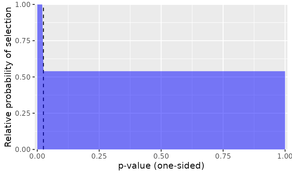
Figure 5: P-value selection probability based on estimated one-step selection model.
Figure 5 illustrates how the likelihood of selection differs as a function of the one-sided \(p\)-value of an effect size estimate. In this example, the plot shows that effect sizes with one-sided \(p\)-values larger than 0.025 are about half as likely \((\lambda_1 = 0.575)\) to be published than effect sizes with smaller \(p\)-values.
See this infographic for additional guidance on interpreting model output from the step-function selection model.
Four-Parameter Step Model with CRVE
Rather than using a single threshold at \(\alpha_1 = 0.025\), we could fit a model that also allows the selection probability for negative effect size estimates to differ from the selection probability for positive but non-significant estimates.
The following code fits such a model, setting steps = c(0.025, 0.500).
We use the same set of weak priors as above.
mod_4PSM <- selection_model(
  data = dat.lehmann2018,
  yi = yi,
  sei = sei,
  cluster = study,
  selection_type = "step",
  steps = c(0.025, 0.500),
  priors = SMD_prior
)

print(mod_4PSM, transf_gamma = TRUE, transf_zeta = TRUE)
## param Est SE p_value CI_lo CI_hi
## beta 0.1083 0.102 0.287 -0.0912 0.308
## tau2 0.0869 0.077 NA 0.0153 0.494
## lambda1 0.6009 0.464 0.509 0.1324 2.727
## lambda2 0.4599 0.391 0.361 0.0870 2.431The estimate of the overall average effect is 0.108, 95% CI [-0.091, 0.308], even smaller than the estimated effect from the three-parameter step model (0.138) and only 50% of the magnitude of the estimate that does not account for selection bias (0.217).
We can visualize the estimated selection function with selection_plot():
selection_plot(mod_4PSM)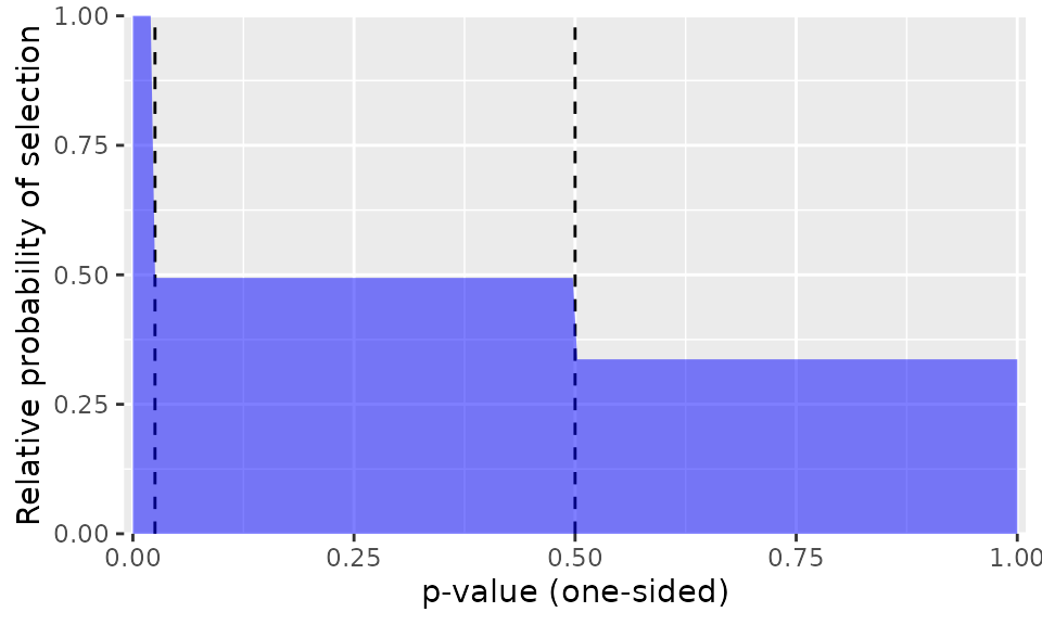
Figure 6: P-value selection probability based on estimated two-step selection model.
As is apparent from Figure 6, this estimated model indicates that negatively signed effects (i.e., those with a one-sided \(p\)-value > 0.50) are even less likely to be observed than effects that are positive but not statistically significant. However, as can be seen from the robust confidence intervals in the model output, the selection parameters are very imprecisely estimated.6
Three-Parameter Step Model with CRVE and Moderators
The selection_model() function allows moderators to be incorporated into model, which enables us to distinguish between systematic study differences and selective reporting bias.
The function allows for both discrete and continuous moderators.
We will use a discrete moderator in this example, specifically whether the study used a within-subjects design compared to a between-subjects design.
We specify the moderator by setting mean_mods = ~ Design.
mod_3PSM_mod <- selection_model(
  data = dat.lehmann2018,
  yi = yi,
  sei = sei,
  cluster = study,
  selection_type = "step",
  steps = 0.025,
  mean_mods = ~ Design,
  priors = SMD_prior
)

mod_3PSM_mod
## param Est SE p_value CI_lo CI_hi
## beta_(Intercept) 0.1196 0.0965 0.215 -0.0694 0.309
## beta_DesignWithin Subjects 0.0822 0.1376 0.550 -0.1875 0.352
## tau2 0.0790 0.0728 NA 0.0130 0.480
## lambda1 0.5631 0.5077 0.524 0.0962 3.297The estimate of the moderator is 0.082, indicating that studies using within-subjects designs have an average effect that is 0.082 larger than studies using between-subjects designs.
The moderator accounts for very little of the between-study variability, as shown by the tau2 estimate, which goes down only slightly from 0.081 to 0.079 when comparing the three-parameter step function model without and with the moderator.
Similarly, the selection parameter lambda_1 remains virtually unchanged (from 0.575 to 0.563).
After taking into account how effects vary based on study design type, effect sizes with one-sided \(p\)-values larger than 0.025 are still about half as likely \((\lambda_1 = 0.563)\) to be published than effect sizes with smaller \(p\)-values.
The evidence-generating process implemented in metaselection also allows for the heterogeneity parameter \(\tau^2\) to be modeled as a function of covariates.
To do so, predictors can be specified using the var_mods argument.
Just like mean_mods, var_mods takes a one-sided formula, following R’s usual syntax for regression specifications.
Beta Function with CRVE
The selection_model() function also allows fitting models based on beta-density selection function by specifying selection_type = "beta".
The default estimator for the beta-density selection model is penalized composite maximum likelihood; the augmented and reweighted Gaussian likelihood estimator is not currently available for this selection model.
In this example, we fit an unpenalized model by explicitly setting priors = NULL.
mod_beta <- selection_model(
  data = dat.lehmann2018,
  yi = yi,
  sei = sei,
  cluster = study,
  selection_type = "beta",
  steps = c(0.025, 0.975),
  priors = NULL
)

print(mod_beta)
## param Est SE p_value CI_lo CI_hi
## beta -0.122 0.125 0.3286 -0.366 0.123
## tau2 0.165 0.150 NA 0.028 0.977
## lambda1 0.910 0.460 0.8522 0.338 2.451
## lambda2 1.610 0.337 0.0231 1.067 2.427The estimate of the overall average effect is -0.122, 95% CI [-0.366, 0.123], which is smaller than both the estimate that does not account for selection bias (0.217) and the estimates from the three- and four-parameter step function models. The average effect estimate based on the beta function is not statistically distinct from zero (\(p\) = 0.329).
To see how the probability of selection differs across studies with different \(p\)-values, we can again visualize the selection function:
selection_plot(mod_beta)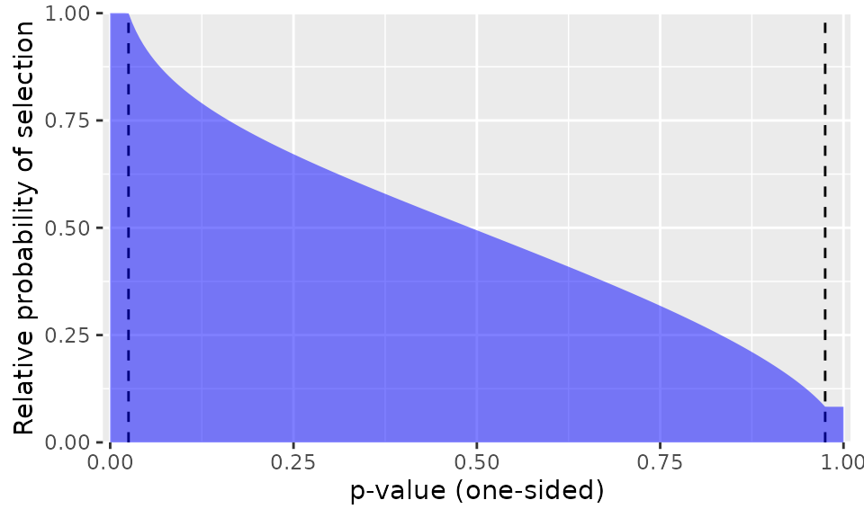
Figure 7: P-value selection probability based on estimated two-step selection model.
Figure 7 shows that effect sizes with smaller \(p\)-values are more likely to be published than effects with larger \(p\)-values. For example, an effect size estimate of zero (with a one-sided \(p\)-value of \(p = 0.500\)) is about half as likely to be published as an effect with a statistically significant, positive effect.
Bootstrap Confidence Intervals
Rather than relying on large-sample CRVE to construct standard errors and confidence intervals for the parameter estimates, it is preferable to instead use confidence intervals based on clustered bootstrap re-sampling.
Simulation results demonstrate that two-stage clustered bootstrapping consistently outperforms CRVE by providing close-to-nominal confidence interval coverage for bias-adjusted average effect sizes (Citkowicz et al., 2026; Pustejovsky et al., 2025).
The code below re-fits the three-parameter step function model to obtain cluster-bootstrap confidence intervals.
We specify bootstrap = "two-stage" to run two-stage cluster bootstrapping and we specify that we want "percentile" bootstrap confidence intervals as the recommended approach.
We specify that number of bootstraps by setting R to 199.
We set the value to 199 here solely to limit the amount of computation.
In practice, we recommend using a much higher number of bootstrap replications, such as 1999, to obtain confidence intervals with more accurate coverage rates (Davidson & MacKinnon, 2000).
We strongly recommend running the selection models with cluster bootstrapping, particularly the two-stage bootstrap with percentile confidence intervals, as this has been shown to improve confidence interval coverage rates relative to using other forms of bootstrap confidence intervals (Pustejovsky et al., 2025).
set.seed(20240916)

system.time(
  mod_3PSM_boot <- selection_model(
    data = dat.lehmann2018,
    yi = yi,
    sei = sei,
    cluster = study,
    selection_type = "step",
    steps = 0.025,
    priors = SMD_prior,
    bootstrap = "two-stage",
    CI_type = "percentile",
    R = 199
  )
)
## user system elapsed
## 58.616 0.018 58.640
print(mod_3PSM_boot, transf_gamma = TRUE, transf_zeta = TRUE)## param Est SE percentile_lower percentile_upper
## beta 0.1382 0.1157 -0.013137 0.403
## tau2 0.0814 0.0763 0.000627 0.215
## lambda1 0.5754 0.5209 0.075718 2.754The overall estimate of the average effect does not change when bootstrapping is applied (0.138). However, the confidence internal is narrower, [-0.013, 0.403] (due partially to the use of a smaller-than-desirable number of bootstrap replications).
Parallel processing
The bootstrapping routine is implemented to work with the future package for parallel processing (Bengtsson, 2021).
For example, the following code specifies a multisession future processing plan with 4 worker nodes, then fits the same model as above:
library(future)
plan(multisession, workers = 4L)

system.time(
  selection_model(
    data = dat.lehmann2018,
    yi = yi,
    sei = sei,
    cluster = study,
    selection_type = "step",
    steps = 0.025,
    bootstrap = "two-stage",
    CI_type = "percentile",
    R = 199
  )
)
## user system elapsed
## 1.512 0.046 9.442Parallel processing substantially reduces the overall computing time. If available, using a larger number of workers would further reduce computing time.
Setting a sequential plan will discontinue use of parallel processing:
plan(sequential)Progress bars
The package is also designed to work with the progressr package (Bengtsson, 2026), which provides customizable progress bars for long-running calculations.
To use a progress bar for only one instance of bootstrapping, wrap the selection_model() call in progressr::with_progress():
library(progressr)

with_progress(
  sel_fit <- selection_model(
    data = dat.lehmann2018,
    yi = yi,
    sei = sei,
    cluster = study,
    selection_type = "step",
    steps = 0.025,
    bootstrap = "two-stage",
    CI_type = "percentile",
    R = 199
  )
)
To turn on progress bars for all bootstrap calculations, use
progressr::handlers(global = TRUE)See vignette("progressr-intro") for further details.